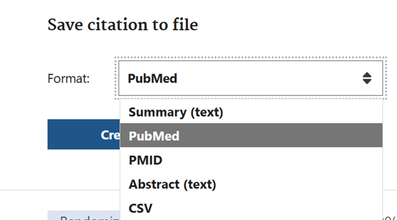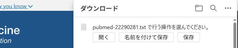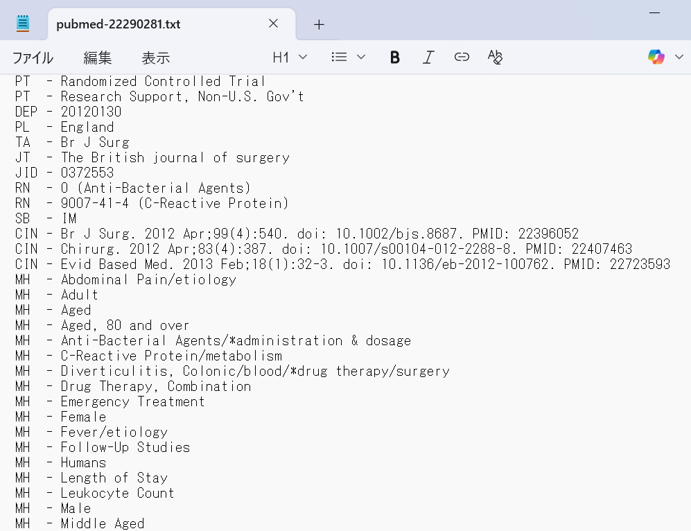
前回の投稿で、PubMed検索の結果をテキストファイルとしてダウンロードする際に、FormatをAbstract (text)にして、アブストラクト情報を含める方法を解説しました。タイトルとアブストラクトにはその論文の最も重要な情報が含まれており、特定のクエスチョンに対して回答を得るのに十分な場合も多いと思います。今回は、GoogleのAIであるGeminiを用いて自分が知りたい情報を引き出せるかを試してみます。GeminiのバージョンはGemini 2.5 Flashです。
知りたい情報とは、例えば、すべての論文をまとめた概略、特定の疑問に対する回答、今まで分析された治療薬の一覧、ランダム化比較試験の対象者の属性、採用基準・除外基準に合致するランダム化比較試験のPICOと効果の要約、などいろいろあるでしょう。
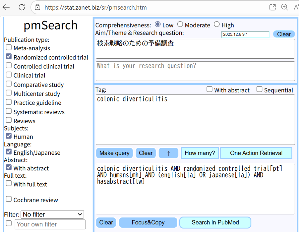
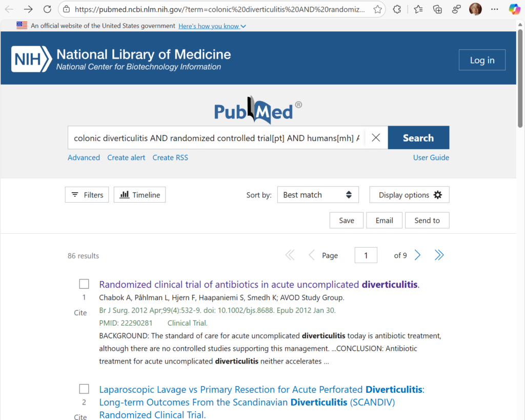
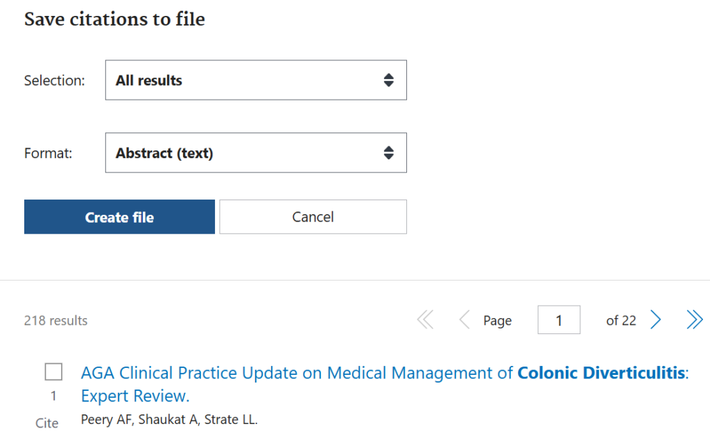
今回は、前回用意した大腸憩室炎に対するランダム化比較試験218件のアブストラクトの情報から臨床に必要な情報を引き出せるか試してみますが、Abstractを含むテキストファイルはかなりの大きさになるので、まずGeminiで扱える情報の大きさを調べてみましょう。
AIでは、取り扱える情報の単位をトークンと呼び、Google Geminiの無料版の場合、1チャットあたり3.2万トークンに制限されています。この制限はコンテキストウインドウと呼ばれます。英語の場合、1トークンは約0.75ワード、日本語の場合は約0.6ワードに相当するそうです。従って、英語の場合32000×0.75=24,000語、2.4万語が限界ということになります。この容量はプロンプトや回答の分も含め、また、続けてプロンプトを実行させる場合はそれらとそれらのプロンプトと回答も含めるということなので、解析対象のテキストファイルのワード数はもっと少なくする必要があります。Geminiで左上にあるチャットを新規作成をクリックして新たにチャットを開始するまでは、加算されていきますので、一連のプロンプトを実行する場合かなり余裕を持って小さめのファイルにする必要があり、PubMed検索結果を対象にするような場合は、無料版のGeminiでは実用的なレベルで使用するのは難しいでしょう。
Googleの提供するNotebookLMでは、アップロードした情報ソースに対してAIで処理ができ、テキストファイルもアップロードできます。1ソースあたり、200MB、50万語、1ノートブックあたり、ソース数50個、ファイルサイズ・単語数は制限なしなので、NotebookLMを使って、同じことができる可能性がありますが、今回はGeminiを使ってやってみます。
今回の大腸憩室炎に対するランダム化比較試験218件のアブストラクトのテキストファイルの大きさは、文献数:218ですが、ファイルサイズ:508KB、ワード数:68,445 、文字数:519,222でした。このサイズは、無料版Geminiでは取り扱える範囲を超えています。Google Workspace Business Standardエディションなどの有料版では、容量が3.2万トークンから100万トークに容量が増えます。NotebookLMで使えるファイル数などもずっと大きくなり、Googleドライブも2TBまで使え、Google Meetなどの機能拡張もあるので、自分はこのGoogle Workspace Business Standardエディションを使っていますので、100万トークン、約70万語の容量まで利用可能です。
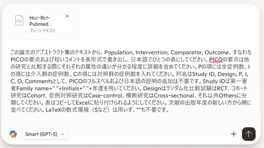
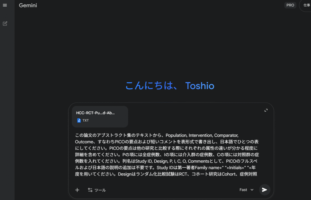
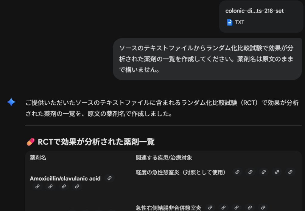
以下に述べるトライアルは2025年12月6日の時点での結果です。思考モード(3 Pro搭載)を使うこともできますが、高速モードを用いていますので先に述べたように、Gemini 2.5 Flashを使っています。まず、Geminiへのプロンプトを入力するフィールドにアブストラクトのテキストファイルをドラグアンドドロップします。ワード数が約6.8万なので、問題なくアップロードできます。(ファイルが大きすぎる場合はアラートが出ます。)それに続けて、以下のプロンプトを書き込み、今までどのような抗生物質がテストされてきたかをまず調べます。
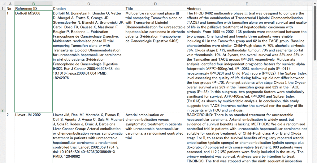
ソースのテキストファイルからランダム化比較試験で効果が分析された薬剤の一覧を作成してください。薬剤名は原文のままで構いません。プロンプトを書き込んで、エンターキーを押すか右向き矢じりをクリックした結果の最初の部分を以下の図に示します。
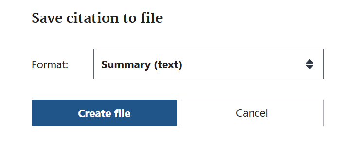
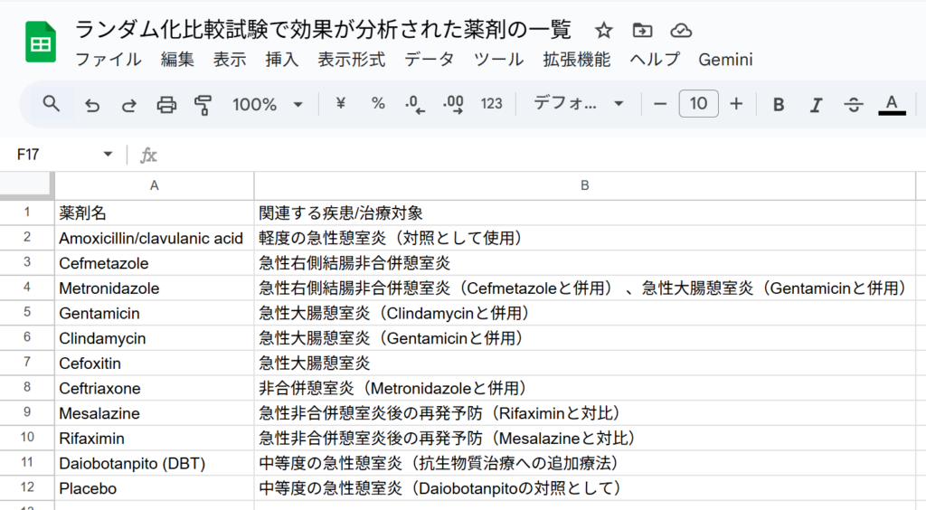
この場合は、”Googleスプレッドシートにエクスポート”のボタンが表示されたので、それをクリックして、Googleスプレッドシートにエクスポートし、ファイル名を書き換えたのが以下の図です。このように、最初にどのような治療法が分析対象になっているかを確認することができます。スプレッドシートに出力したい場合、追加のプロンプトで”表をスプレッドシートにエクスポートできるように作成してください。”と書くことで、CSVファイルとして保存できるデータが出力されるので、これをテキストエディタにコピーして貼り付けて.csvの拡張子で保存し、そのファイルをGoogleスプレッドシートやExcelでインポートする方法が使えます。
また、Geminiは注記として、以下の説明を出力しました。
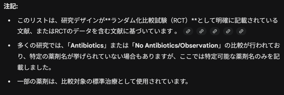
Abstractの情報に基づいているので、必ずしもすべての抗菌薬の名称が明らかになるわけではありませんということです。
試しに、Levofloxacinの効果について聞いてみることにしました。PICO要約表を作成するように指示しており、採用基準と除外基準を設定して、ランダム化比較試験に限定するよう指示しています。このプロンプトは採用基準と除外基準を書き換えることで、プロトタイプとして、他のクエスチョンにも使えるはずです。
ソースのテキストファイルから、以下の採用基準と除外基準に合致する文献を抽出して、Study ID、P、I、C、O、コメント、PMIDの7列からなる表を作成してください。
Study IDは第一著者の姓のフルスペル+半角スペース+イニシャル+半角スペース+年度を記述してください。
Pの欄は対象者に関する記述(症例数)、Iの欄は介入に関する記述(症例数)、Cの欄は対照の治療に関する記述(症例数)、Oの欄は測定されたアウトカムの内容を記述してください。
コメント蘭は効果の概略を記述してください。
PMIDの欄はhttps://pubmed.ncbi.nlm.nih.gov/PMID/のように、クリックしたらPubMedの該当する文献を開けるようなリンクのURLを記述してください。
P, I, C, Oの欄は他の研究との違いが分かる程度の詳細な情報を含めてください。研究は年度の新しい順に並べ、Googleスプレッドシートへエクスポートできる形式で提示してください。
採用基準:
研究デザインはランダム化比較試験。
対象は成人の大腸憩室炎の患者。
介入がLevofloxacin。
対照がプラセボあるいは無治療あるいは保存的治療。
治癒をアウトカムとして分析。
除外基準:
システマティックレビュー/メタアナリシスの論文は除外する。
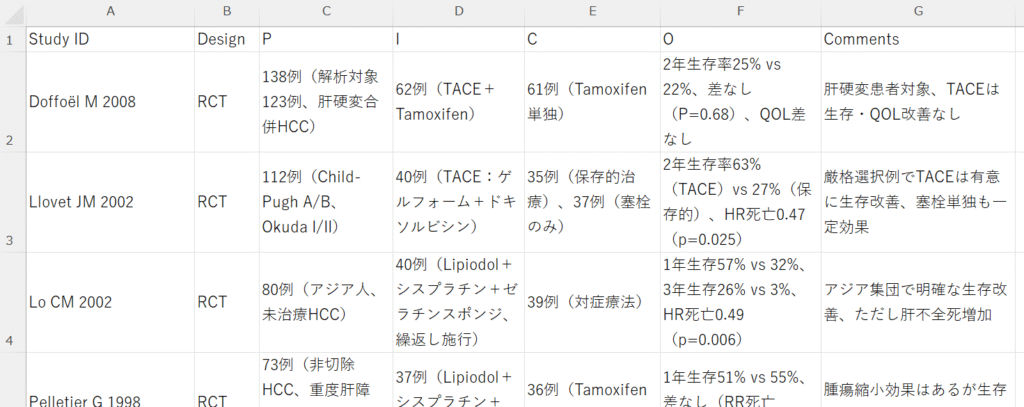
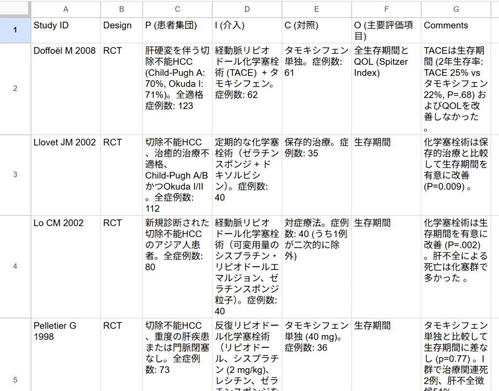
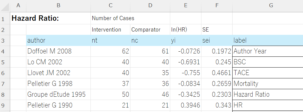
対象が小児患者は除外する。当然のことながら、Levofloxacinを治療薬として使用しているランダム化比較試験は見つからないと回答し、使用された抗生物質をリストアップして、「介入がLevofloxacin」という基準を除外し、「抗生物質群と無抗生物質(または非観察的/非手術的)群を比較した成人非合併大腸憩室炎を対象とするランダム化比較試験(RCT)」を抽出した参考情報としての表を出力した、と回答しています。表の部分ををCSVファイルとして保存し、さらにGoogleスプレッドシートにインポートして形式を整えた画面が以下の図です。
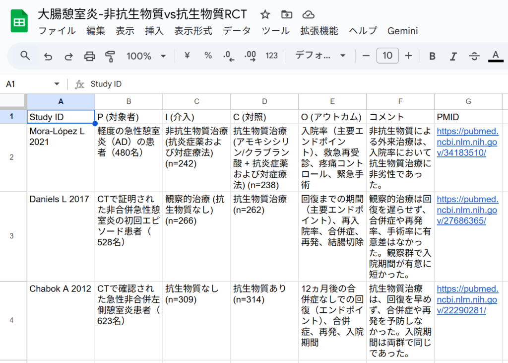
IとCの部分を見ると、介入Iの方が抗生物質なしになっており、対照Cの方が抗生物質治療になっていて、非劣性試験も含まれています。結果は、少なくとも軽症の急性憩室炎では、抗生物質は観察的治療と比べ差がないことが示されています。これだけからも、大腸憩室炎に対して抗生物質による治療が必要ないということが最近の潮流ではないかということがうかがい知れます。
PMIDの部分のURLをクリックするとPubMedでその文献のアブストラクトが表示されるので、それぞれのアブストラクト情報を確認することができます。
さらに、診療ガイドラインの情報が含まれているか聞いてみました。
ソースに診療ガイドラインは含まれていますか?AGAのアップデート、ドイツ消化器病・代謝疾患学会およびドイツ一般・内臓外科学会の憩室疾患に関するガイドライン、デンマークの治療ガイドライン、オランダ社会のガイドラインが引用され、SAGES ホワイトペーパーについて次のように記述されていました:SAGES ホワイトペーパー これは、抗生物質の非ルーチン使用に関するエビデンスをレビューし、安全な実施方法を検討したものです 。
さらに、また、治療アルゴリズムや伝統的なパラダイムの変化を議論し、臨床的推奨に影響を与える以下の文献も含まれています、との記述が続き、文献が引用されていました。そして、これらの文書は、大腸憩室炎の診断、内科的・外科的治療、および再発予防に関する従来の慣行が変化していることを示しており 、特に非合併急性憩室炎に対する抗生物質の非ルーチン使用が最新の推奨事項であることを裏付けています、との記述がありました。
これらの回答から、大腸憩室炎に対して抗生物質をルーチンで投与することは必要ないことが分かってきます。そこで、対象者について以下のプロンプトでさらに確認してみましょう。
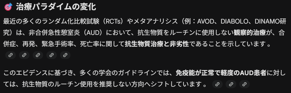
抗生物質非ルーチン使用の対象となる大腸憩室炎患者の条件は?抗生物質の非ルーチン使用(すなわち、抗生物質を投与しない観察的治療)の対象となる大腸憩室炎患者の条件は、主に非合併急性憩室炎(AUD)の患者です 、との回答に続き、憩室炎のタイプ、免疫状態・全身状態、画像診断による評価について詳細が示され、さらに、非推奨/注意が必要な患者(抗生物質が推奨される場合)について回答が続きます。そして、最後に治療パラダイムの変化の解説がありました。
218件の文献のアブストラクトを全部読む時間と労力に比べると、あっという間にこのような情報が得られます。
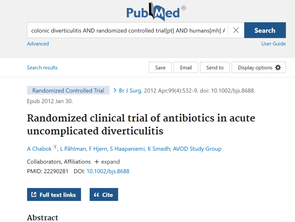
今回Geminiの回答が正確かどうかについて確認するひとつの方法として、診療ガイドラインを参照することが考えられます。AGAの診療ガイドラインの論文についてPMIDをGeminiに聞いて、その論文を見てみることにします。この論文です: Peery AF, Shaukat A, Strate LL: AGA Clinical Practice Update on Medical Management of Colonic Diverticulitis: Expert Review. Gastroenterology 2021;160:906-911.e1. doi: 10.1053/j.gastro.2020.09.059 PMID: 33279517
この論文のアブストラクトには”Antibiotic treatment can be used selectively rather than routinely in immunocompetent patients with mild acute uncomplicated diverticulitis. Antibiotic treatment is strongly advised in immunocompromised patients.”と明確に書かれており、Geminiの回答は正確であると言っていいと思われます。また、この論文のPubMedのアブストラクトのページには、Full text linksもあるので、必要ならさらに全文を目を通してGeminiの回答が正しいかを確認することもできます。
最後に、「抗生物質非ルーチン使用の対象となる大腸憩室炎患者の条件は?」に対するGeminiの回答の詳細を提示しておきます。
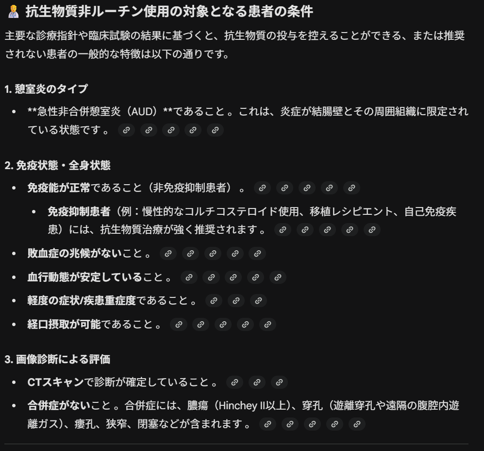
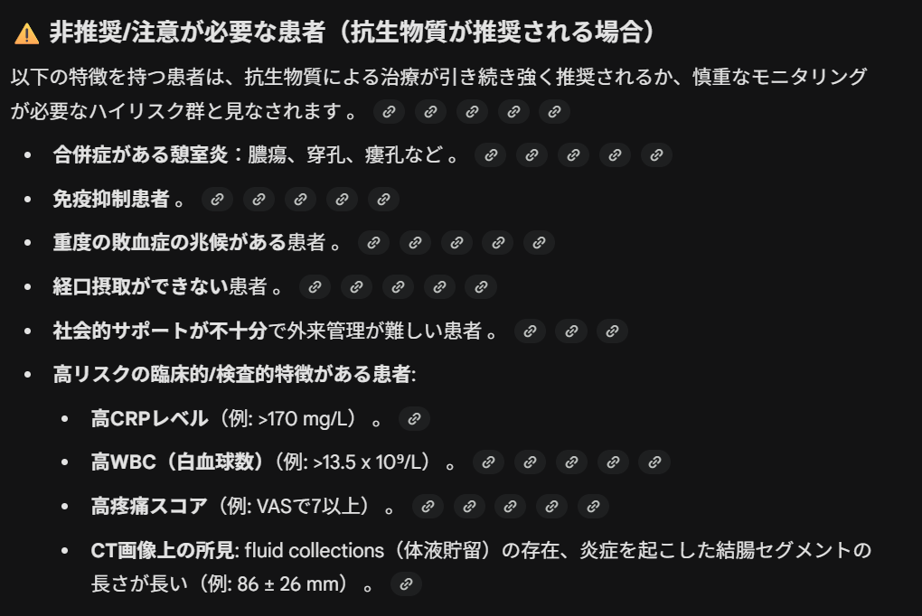
かなり詳細な情報なので、実際の症例に抗生物質を投与すべきかどうかの判断に使えると考えられます。
今回の例から、PubMedの検索結果からランダム化比較試験のアブストラクト情報を得て、Geminiを利用することで、極めて短時間で臨床に必要な情報が得られることが分かりました。また、PICO要約表を作成することもできるので、システマティックレビュー/メタアナリシスの文献選定にも使える可能性があることが分かりました。