以前の投稿「Stanを使うベイジアンアプローチのメタアナリシス:Copilotに聞きながら」でRからrstanを介してStanを動かし、メタアナリシスを実行するまでの過程を紹介しました。
今回、リスク比、オッズ比、リスク差を効果指標とするメタアナリシスを実行し、Forest plotを出力するまでの、スクリプトを作成しました。
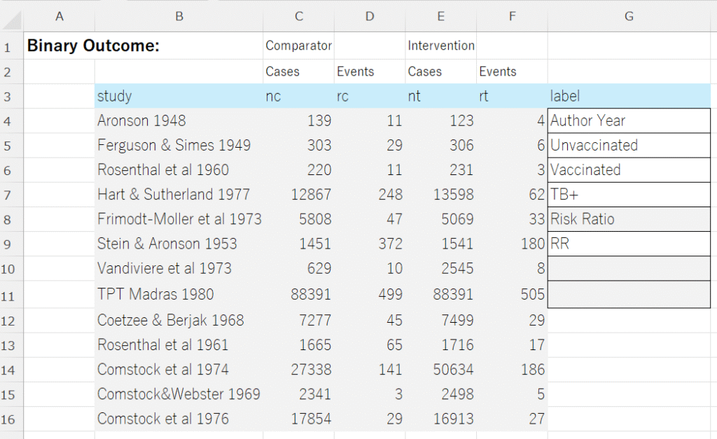
データは、図に示すような形式でExcelで用意します。Risk Ratio、RRのセルをOdds Ratio、ORあるいはRisk Difference、 RDと書き換えて効果指標のタイプを指定します。labelのその他の項目もそれぞれ書き換えてください。この例ではUnvaccinatedのセルが対照の治療、Vaccinatedのセルが介入の治療、TB+のセルがアウトカムになります。効果指標のタイプはRR, OR, RDのラベル名で判断します。
この例では、セルB3からG16の範囲を選択して(データ部分が例えば行7までしかない場合は、セルB3からセルG9の範囲を選択します)、以下のスクリプトをRで実行するとForest plotが出力されます。かなり長いのでアコーディオン形式で畳んだ状態ですが、右端をクリックすると展開され、コード用のフィールドに記述してあります。
コードをすべて、コピーして、RのEditorに貼り付けます。Excelでデータ範囲を選択し、コピー(Ctrl+C)の後、Rに戻り、exdat = read.delim(“clipboard”,sep=”\t”,header=TRUE)の行のスクリプトを実行して、クリップボード経由でデータを読み込みます。その後、それ以降のスクリプトをすべて実行します。
Stanを用いるベイジアンメタアナリシス用コード
#####rstan, StanによるRR, OR, RDのベイジアンメタアナリシス用のスクリプト#####
# 必要なパッケージをロード
library(rstan)
library(bayesplot)
library(dplyr)
library(HDInterval)
library(forestplot)
library(metafor)
# Get data via clipboard.
exdat = read.delim("clipboard",sep="\t",header=TRUE)
labem = exdat[,"label"]
em = labem[6]
labe_study = labem[1]
labe_cont = labem[2]
labe_int = labem[3]
labe_outc = labem[4]
labe_em = labem[5]
# Format the data.
exdati = na.omit(exdat)
if(colnames(exdati)[1]=="author"){
study = exdati$author
}
if(colnames(exdati)[1]=="study"){
study = exdati$study
}
nc = exdati$nc
rc = exdati$rc
nt = exdati$nt
rt = exdati$rt
num_studies = length(study)
N = num_studies
meta_data <- list(
N = num_studies,
study = study,
nc = nc,
rc = rc,
nt = nt,
rt = rt
)
# Stanモデルコード
#RR
if(em == "RR"){
stan_model_code <- "data {
int<lower=1> N;
int nc[N];
int rc[N];
int nt[N];
int rt[N];
}
parameters {
// リスク比 (RR) 用
real logRR[N];
real mu_logRR; // リスク比の統合値(対数)
real<lower=0> sigma_logRR; // リスク比の研究間のばらつき
real<lower=0, upper=1> p_c[N]; // 対照群のイベント発生確率
}
transformed parameters { // 各研究のlogRR, logOR, RDをここに定義
vector[N] logRR_study; // 各研究のlogRR
for (i in 1:N) {
// これらの値はmu_logRRなどからサンプリングされるものですが、
// ここで直接観測データから計算された「点推定値」も用意します
// これらはgenerated quantitiesでしか使わないので、generated quantitiesに移すことも可能
// ただし、modelブロックで使われている logRR[i] 等と重複しないように注意
// ここでは、計算の便宜上、rc,nc,rt,nt から直接点推定値を計算します
real p_c_obs = (rc[i] + 0.5) / (nc[i] + 1.0); // ゼロイベント回避のための補正
real p_t_obs = (rt[i] + 0.5) / (nt[i] + 1.0);
logRR_study[i] = log(p_t_obs) - log(p_c_obs);
}
}
model {
// 事前分布
// RR
mu_logRR ~ normal(0, 10);
sigma_logRR ~ cauchy(0, 2);
for (i in 1:N) {
p_c[i] ~ beta(1, 1); // 対照群のイベント発生確率に対する一様な事前分布
// RR
logRR[i] ~ normal(mu_logRR, sigma_logRR);
rc[i] ~ binomial(nc[i], p_c[i]);
rt[i] ~ binomial(nt[i], fmin(p_c[i] * exp(logRR[i]), 1)); // RRに基づき介入群のイベント率を計算
}
}
generated quantities {
// リスク比 (RR)
real RR_pooled = exp(mu_logRR);
real RR_pred = exp(normal_rng(mu_logRR, sigma_logRR));
real tau_squared_logRR = sigma_logRR * sigma_logRR;
// 各研究の観測された効果量の標準誤差 (se_obs) を計算
vector<lower=0>[N] se_logRR_obs;
// 各効果指標の観測誤差の分散 (variance_obs)
vector<lower=0>[N] variance_logRR_obs;
// 典型的な研究内分散 (S_squared)
real S_squared_logRR;
for (i in 1:N) {
// ゼロイベント/総数ゼロを避けるために、0.5の連続性補正を適用
// 頻度論的なメタアナリシスでよく使われる手法です。
real current_rc = rc[i] + 0.5;
real current_nc = nc[i] + 1.0;
real current_rt = rt[i] + 0.5;
real current_nt = nt[i] + 1.0;
// logRR の標準誤差の計算 (デルタ法)
se_logRR_obs[i] = sqrt(1.0/current_rc - 1.0/current_nc + 1.0/current_rt - 1.0/current_nt);
variance_logRR_obs[i] = se_logRR_obs[i] * se_logRR_obs[i];
}
// 典型的な研究内分散 (S_squared) の計算
// 各研究の観測誤差の分散の平均値
S_squared_logRR = mean(variance_logRR_obs);
}"
}
#OR
if(em == "OR"){
stan_model_code <- "data {
int<lower=1> N;
int nc[N];
int rc[N];
int nt[N];
int rt[N];
}
parameters {
// オッズ比 (OR) 用
real logOR[N];
real mu_logOR; // オッズ比の統合値(対数)
real<lower=0> sigma_logOR; // オッズ比の研究間のばらつき
real<lower=0, upper=1> p_c[N]; // 対照群のイベント発生確率
}
transformed parameters { // 各研究のlogRR, logOR, RDをここに定義
vector[N] logOR_study; // 各研究のlogOR
for (i in 1:N) {
// これらの値はmu_logRRなどからサンプリングされるものですが、
// ここで直接観測データから計算された「点推定値」も用意します
// これらはgenerated quantitiesでしか使わないので、generated quantitiesに移すことも可能
// ただし、modelブロックで使われている logRR[i] 等と重複しないように注意
// ここでは、計算の便宜上、rc,nc,rt,nt から直接点推定値を計算します
real p_c_obs = (rc[i] + 0.5) / (nc[i] + 1.0); // ゼロイベント回避のための補正
real p_t_obs = (rt[i] + 0.5) / (nt[i] + 1.0);
logOR_study[i] = log((p_t_obs / (1 - p_t_obs))) - log((p_c_obs / (1 - p_c_obs)));
}
}
model {
// 事前分布
// OR
mu_logOR ~ normal(0, 10);
sigma_logOR ~ cauchy(0, 2);
for (i in 1:N) {
p_c[i] ~ beta(1, 1); // 対照群のイベント発生確率に対する一様な事前分布
// OR
logOR[i] ~ normal(mu_logOR, sigma_logOR);
rc[i] ~ binomial(nc[i], p_c[i]);
// オッズ比の定義 p_t / (1 - p_t) = OR * (p_c / (1 - p_c)) より p_t を導出
// logit(p_t) = logOR + logit(p_c)
// p_t = inv_logit(logOR + logit(p_c))
rt[i] ~ binomial(nt[i], inv_logit(logOR[i] + logit(p_c[i])));
}
}
generated quantities {
// オッズ比 (OR)
real OR_pooled = exp(mu_logOR);
real OR_pred = exp(normal_rng(mu_logOR, sigma_logOR));
real tau_squared_logOR = sigma_logOR * sigma_logOR;
// 各研究の観測された効果量の標準誤差 (se_obs) を計算
vector<lower=0>[N] se_logOR_obs;
// 各効果指標の観測誤差の分散 (variance_obs)
vector<lower=0>[N] variance_logOR_obs;
// 典型的な研究内分散 (S_squared)
real S_squared_logOR;
for (i in 1:N) {
// ゼロイベント/総数ゼロを避けるために、0.5の連続性補正を適用
// 頻度論的なメタアナリシスでよく使われる手法です。
real current_rc = rc[i] + 0.5;
real current_nc = nc[i] + 1.0;
real current_rt = rt[i] + 0.5;
real current_nt = nt[i] + 1.0;
// logOR の標準誤差の計算 (デルタ法)
se_logOR_obs[i] = sqrt(1.0/current_rc + 1.0/(current_nc - current_rc) + 1.0/current_rt + 1.0/(current_nt - current_rt));
variance_logOR_obs[i] = se_logOR_obs[i] * se_logOR_obs[i];
}
// 典型的な研究内分散 (S_squared) の計算
// 各研究の観測誤差の分散の平均値
S_squared_logOR = mean(variance_logOR_obs);
}"
}
#RD
if(em == "RD"){
stan_model_code <- "data {
int<lower=1> N;
int nc[N];
int rc[N];
int nt[N];
int rt[N];
}
parameters {
// リスク差 (RD) 用
real RD[N];
real mu_RD; // リスク差の統合値
real<lower=0> sigma_RD; // リスク差の研究間のばらつき
real<lower=0, upper=1> p_c[N]; // 対照群のイベント発生確率
}
transformed parameters { // 各研究のlogRR, logOR, RDをここに定義
vector[N] RD_study; // 各研究のRD
for (i in 1:N) {
// これらの値はmu_logRRなどからサンプリングされるものですが、
// ここで直接観測データから計算された「点推定値」も用意します
// これらはgenerated quantitiesでしか使わないので、generated quantitiesに移すことも可能
// ただし、modelブロックで使われている logRR[i] 等と重複しないように注意
// ここでは、計算の便宜上、rc,nc,rt,nt から直接点推定値を計算します
real p_c_obs = (rc[i] + 0.5) / (nc[i] + 1.0); // ゼロイベント回避のための補正
real p_t_obs = (rt[i] + 0.5) / (nt[i] + 1.0);
RD_study[i] = p_t_obs - p_c_obs;
}
}
model {
// 事前分布
// RD
mu_RD ~ normal(0, 10);
sigma_RD ~ cauchy(0, 2);
for (i in 1:N) {
p_c[i] ~ beta(1, 1); // 対照群のイベント発生確率に対する一様な事前分布
// RD
RD[i] ~ normal(mu_RD, sigma_RD);
rc[i] ~ binomial(nc[i], p_c[i]);
// リスク差の定義 p_t - p_c = RD より p_t を導出
// p_t = p_c + RD
rt[i] ~ binomial(nt[i], fmin(fmax(p_c[i] + RD[i], 0), 1)); // 0から1の範囲に制限
}
}
generated quantities {
// リスク差 (RD)
real RD_pooled = mu_RD;
real RD_pred = normal_rng(mu_RD, sigma_RD);
real tau_squared_RD = sigma_RD * sigma_RD;
// 各研究の観測された効果量の標準誤差 (se_obs) を計算
vector<lower=0>[N] se_RD_obs;
// 各効果指標の観測誤差の分散 (variance_obs)
vector<lower=0>[N] variance_RD_obs;
// 典型的な研究内分散 (S_squared)
real S_squared_RD;
for (i in 1:N) {
// ゼロイベント/総数ゼロを避けるために、0.5の連続性補正を適用
// 頻度論的なメタアナリシスでよく使われる手法です。
real current_rc = rc[i] + 0.5;
real current_nc = nc[i] + 1.0;
real current_rt = rt[i] + 0.5;
real current_nt = nt[i] + 1.0;
// RD の標準誤差の計算 (デルタ法)
// p_c = rc/nc, p_t = rt/nt
// var(RD) = var(p_t - p_c) = var(p_t) + var(p_c) (独立と仮定)
// var(p) = p*(1-p)/n
real p_c_calc = current_rc / current_nc;
real p_t_calc = current_rt / current_nt;
se_RD_obs[i] = sqrt(p_c_calc * (1.0 - p_c_calc) / current_nc + p_t_calc * (1.0 - p_t_calc) / current_nt);
variance_RD_obs[i] = se_RD_obs[i] * se_RD_obs[i];
}
// 典型的な研究内分散 (S_squared) の計算
// 各研究の観測誤差の分散の平均値
S_squared_RD = mean(variance_RD_obs);
}"
}
# 初期値の設定
N <- meta_data$N
init_values <- function() {
list(
mu_logRR = 0, sigma_logRR = 1, logRR = rep(0, N),
mu_logOR = 0, sigma_logOR = 1, logOR = rep(0, N),
mu_RD = 0, sigma_RD = 1, RD = rep(0, N),
p_c = rep(0.1, N)
)
}
# Stanモデルのコンパイルと実行
# ウォームアップ10000回、サンプリングは20000回x4チェインで80000個に設定。適宜変更する。
fit <- stan(model_code = stan_model_code, data = meta_data, init = init_values, iter = 30000, warmup=10000, chains = 4, seed = 123,control = list(adapt_delta = 0.98))
#fit <- stan(model_code = stan_model_code, data = meta_data, init = init_values, iter = 30000, warmup=10000, chains = 4, seed = 123)
# 推定結果の抽出
posterior_samples <- extract(fit)
# --- 結果の表示 ---
## リスク比 (RR)
if(em == "RR"){
cat("--- リスク比 (RR) の結果 ---\n")
mu_logRR_samples <- posterior_samples$mu_logRR
risk_ratio <- exp(mean(mu_logRR_samples))
conf_int_rr <- exp(quantile(mu_logRR_samples, probs = c(0.025, 0.975)))
pi_rr = quantile(posterior_samples$RR_pred, probs = c(0.025, 0.975)) #PI of RR
p_val_rr = round(2*min(mean(mu_logRR_samples >0), mean(mu_logRR_samples <0)), 6) #Bayesian p-value for summary logRR
if(mean(mu_logRR_samples)>0){
prob_direct_rr = round(mean(mu_logRR_samples > 0),6)
label = "p(RR>1)="
}else{
prob_direct_rr = round(mean(mu_logRR_samples < 0),6)
label = "p(RR<1)="
}
cat("推定されたリスク比:", risk_ratio, "\n")
cat("95% 確信区間:", conf_int_rr[1], "-", conf_int_rr[2]," P=",p_val_rr,label,prob_direct_rr,"\n\n")
cat("95% 推測区間:", pi_rr[1], "-", pi_rr[2])
}
if(em == "OR"){
## オッズ比 (OR)
cat("--- オッズ比 (OR) の結果 ---\n")
mu_logOR_samples <- posterior_samples$mu_logOR
odds_ratio <- exp(mean(mu_logOR_samples))
conf_int_or <- exp(quantile(mu_logOR_samples, probs = c(0.025, 0.975)))
pi_or = quantile(posterior_samples$OR_pred, probs = c(0.025, 0.975)) #PI of OR
p_val_or = round(2*min(mean(mu_logOR_samples >0), mean(mu_logOR_samples <0)), 6) #Bayesian p-value for summary logOR
if(mean(mu_logOR_samples)>0){
prob_direct_or = round(mean(mu_logOR_samples > 0),6)
label = "p(OR>1)="
}else{
prob_direct_or = round(mean(mu_logOR_samples < 0),6)
label = "p(OR<1)="
}
cat("推定されたオッズ比:", odds_ratio, "\n")
cat("95% 確信区間:", conf_int_or[1], "-", conf_int_or[2]," P=",p_val_or,label,prob_direct_or, "\n\n")
cat("95% 推測区間:", pi_or[1], "-", pi_or[2])
}
if(em == "RD"){
## リスク差 (RD)
cat("--- リスク差 (RD) の結果 ---\n")
mu_RD_samples <- posterior_samples$mu_RD
risk_difference <- mean(mu_RD_samples)
conf_int_rd <- quantile(mu_RD_samples, probs = c(0.025, 0.975))
pi_rd = quantile(posterior_samples$RD_pred, probs = c(0.025, 0.975)) #PI of RD
p_val_rd = round(2*min(mean(mu_RD_samples >0), mean(mu_RD_samples <0)), 6) #Bayesian p-value for summary RD
if(mean(mu_RD_samples)>0){
prob_direct_rd = round(mean(mu_RD_samples > 0),6)
label = "p(RD>0)="
}else{
prob_direct_rd = round(mean(mu_RD_samples < 0),6)
label = "p(RD<0)="
}
cat("推定されたリスク差:", risk_difference, "\n")
cat("95% 確信区間:", conf_int_rd[1], "-", conf_int_rd[2]," P=",p_val_rd,label,prob_direct_rd, "\n")
cat("95% 推測区間:", pi_rd[1], "-", pi_rd[2])
}
#######
#各研究の効果指標と95%確信区間の値
if(em == "RR"){
# リスク比
rr=rep(0,N)
rr_lw=rep(0,N)
rr_up=rep(0,N)
for(i in 1:N){
rr[i] = exp(mean(posterior_samples$logRR[,i]))
rr_lw[i] = exp(quantile(posterior_samples$logRR[,i],probs=0.025))
rr_up[i] = exp(quantile(posterior_samples$logRR[,i],probs=0.975))
}
}
if(em == "OR"){
#オッズ比
or=rep(0,N)
or_lw=rep(0,N)
or_up=rep(0,N)
for(i in 1:N){
or[i] = exp(mean(posterior_samples$logOR[,i]))
or_lw[i] = exp(quantile(posterior_samples$logOR[,i],probs=0.025))
or_up[i] = exp(quantile(posterior_samples$logOR[,i],probs=0.975))
}
}
if(em == "RD"){
#リスク差
rd=rep(0,N)
rd_lw=rep(0,N)
rd_up=rep(0,N)
for(i in 1:N){
rd[i] = mean(posterior_samples$RD[,i])
rd_lw[i] = quantile(posterior_samples$RD[,i],probs=0.025)
rd_up[i] = quantile(posterior_samples$RD[,i],probs=0.975)
}
}
#####
#####I-squared:
if(em == "RR"){
# --- リスク比 (logRR) の I-squared 計算 ---
tau_squared_logRR_samples <- posterior_samples$tau_squared_logRR
S_squared_logRR_from_stan <- posterior_samples$S_squared_logRR[1] # S_squaredは各イテレーションで同じ値なので、最初の要素でOK
# 各イテレーションでI-squaredを計算
I_squared_logRR_samples <- (tau_squared_logRR_samples / (tau_squared_logRR_samples + S_squared_logRR_from_stan)) * 100
# I-squaredの点推定値(平均値)と95%確信区間を計算
#mean_I_squared_logRR <- mean(I_squared_logRR_samples)
#ci_I_squared_logRR <- quantile(I_squared_logRR_samples, probs = c(0.025, 0.975))
#mode and HDI (high density interval) RR
dens=density(I_squared_logRR_samples)
mean_I_squared_logRR=dens$x[which.max(dens$y)] #mode
ci_I_squared_logRR=hdi(I_squared_logRR_samples) #High Density Interval (HDI) lower and upper.
cat(paste0("--- I-squared for Log Relative Risk ---\n"))
cat(paste0("Estimated I-squared (Mode): ", round(mean_I_squared_logRR, 2), "%\n"))
cat(paste0("95% High Density Interval for I-squared: ", round(ci_I_squared_logRR[1], 2), "% - ", round(ci_I_squared_logRR[2], 2), "%\n"))
}
if(em == "OR"){
# --- オッズ比 (logOR)ついても同様に計算 ---
tau_squared_logOR_samples <- posterior_samples$tau_squared_logOR
S_squared_logOR_from_stan <- posterior_samples$S_squared_logOR[1] # S_squaredは各イテレーションで同じ値なので、最初の要素でOK
# ... 同様の計算 ...
# 各イテレーションでI-squaredを計算
I_squared_logOR_samples <- (tau_squared_logOR_samples / (tau_squared_logOR_samples + S_squared_logOR_from_stan)) * 100
# I-squaredの点推定値(平均値)と95%確信区間を計算
#mean_I_squared_logOR <- mean(I_squared_logOR_samples)
#ci_I_squared_logOR <- quantile(I_squared_logOR_samples, probs = c(0.025, 0.975))
#mode and HDI (High Density Interval) OR
dens=density(I_squared_logOR_samples)
mean_I_squared_logOR=dens$x[which.max(dens$y)] #mode
ci_I_squared_logOR=hdi(I_squared_logOR_samples) #High Density Interval (HDI) lower and upper.
cat(paste0("--- I-squared for Log Odds Ratio ---\n"))
cat(paste0("Estimated I-squared (Mode): ", round(mean_I_squared_logOR, 2), "%\n"))
cat(paste0("95% High Density Interval for I-squared: ", round(ci_I_squared_logOR[1], 2), "% - ", round(ci_I_squared_logOR[2], 2), "%\n"))
}
if(em == "RD"){
# --- リスク差 (RD) についても同様に計算 ---
tau_squared_RD_samples <- posterior_samples$tau_squared_RD
S_squared_RD_from_stan <- posterior_samples$S_squared_RD[1] # S_squaredは各イテレーションで同じ値なので、最初の要素でOK
# ... 同様の計算 ...
# 各イテレーションでI-squaredを計算
I_squared_RD_samples <- (tau_squared_RD_samples / (tau_squared_RD_samples + S_squared_RD_from_stan)) * 100
# I-squaredの点推定値(平均値)と95%確信区間を計算
#mean_I_squared_RD <- mean(I_squared_RD_samples)
#ci_I_squared_RD <- quantile(I_squared_RD_samples, probs = c(0.025, 0.975))
#mode and HDI (High Density Interval) RD
dens=density(I_squared_RD_samples)
mean_I_squared_RD=dens$x[which.max(dens$y)] #mode
ci_I_squared_RD=hdi(I_squared_RD_samples) #High Density Interval (HDI) lower and upper.
cat(paste0("--- I-squared for Risk Difference ---\n"))
cat(paste0("Estimated I-squared (Mode): ", round(mean_I_squared_RD, 2), "%\n"))
cat(paste0("95% High Density Interval for I-squared: ", round(ci_I_squared_RD[1], 2), "% - ", round(ci_I_squared_RD[2], 2), "%\n"))
}
#####
####MCMC diagnostic####
#MCMC trace plot: logRR
#dev.new();mcmc_dens(as.matrix(fit, pars = c("logRR","tau_squared_logRR")))
#dev.new();mcmc_trace(fit, pars = c("mu_logRR", "sigma_logRR"))
#Pairs plot
#dev.new();mcmc_pairs(fit, pars = c("mu_logRR", "sigma_logRR"))
#### Forest plot #####
#Risk Ratio (RR)
if(em == "RR"){
# 重みを格納するベクトルを初期化
weights <- numeric(N)
weight_percentages <- numeric(N)
for (i in 1:N) {
# i番目の研究のlogRRのサンプリング値を取得
log_RR_i_samples <- posterior_samples$logRR[, i]
# そのサンプリングされた値の分散を計算
# これを「実効的な逆分散」と考える
variance_of_logRR_i <- var(log_RR_i_samples)
# 重みは分散の逆数
weights[i] <- 1 / variance_of_logRR_i
}
# 全重みの合計
total_weight <- sum(weights)
# 各研究の重みのパーセンテージ
weight_percentages <- (weights / total_weight) * 100
# 結果の表示
results_weights_posterior_var <- data.frame(
Study = 1:N,
Effective_Weight = weights,
Effective_Weight_Percentage = weight_percentages
)
print(results_weights_posterior_var)
k=N
wpc = format(round(weight_percentages,digits=1), nsmall=1)
wp = weight_percentages/100
#Forest plot box sizes on weihts
wbox=c(NA,NA,(k/4)*sqrt(wp)/sum(sqrt(wp)),0.5,0,NA)
#wbox=c(NA,NA,(k/5)*sqrt(wp)/sum(sqrt(wp)),0.5,0,NA)
###### tau-squared
# logRR の tau^2
tau_squared_logRR_samples <- posterior_samples$tau_squared_logRR
#mean_tau_squared_logRR <- mean(tau_squared_logRR_samples)
#ci_tau_squared_logRR <- quantile(tau_squared_logRR_samples, probs = c(0.025, 0.975))
#mode and HDI (High Density Interval) logRR tau-squared
dens=density(tau_squared_logRR_samples)
mean_tau_squared_logRR=dens$x[which.max(dens$y)] #mode
ci_tau_squared_logRR=hdi(tau_squared_logRR_samples) #High Density Interval (HDI) lower and upper.
print(paste("Estimated tau-squared (logRR, mode):", mean_tau_squared_logRR))
print(paste("95% High Density Interval for tau-squared (logRR):", ci_tau_squared_logRR[1], "-", ci_tau_squared_logRR[2]))
#Forest plot by forestplot
#setting fs for cex
fs=1
if(k>20){fs=round((1-0.02*(k-20)),digits=1)}
m=c(NA,NA,rr,risk_ratio,risk_ratio,NA)
lw=c(NA,NA,rr_lw,conf_int_rr[1],pi_rr[1],NA)
up=c(NA,NA,rr_up,conf_int_rr[2],pi_rr[2],NA)
hete1=""
hete2=paste("I2=",round(mean_I_squared_logRR, 2),"%",sep="")
hete3=paste("tau2=",format(round(mean_tau_squared_logRR,digits=4),nsmall=4),sep="")
#hete2=paste("I2=",round(mean_I_squared_logRR, 2), "%\n"," (",round(ci_I_squared_logRR[1], 2)," ~ ",
#round(ci_I_squared_logRR[2], 2),")",sep="")
#hete3=paste("tau2=",format(round(mean_tau_squared_logRR,digits=4),nsmall=4), "\n",
#" (",format(round(ci_tau_squared_logRR[1],digits=4),nsmall=4)," ~ ",
#format(round(ci_tau_squared_logRR[2],digits=4),nsmall=4),") ",sep="")
hete4=""
hete5=paste("p=",p_val_rr, sep="")
hete6=paste(label,prob_direct_rr,sep="")
au=study
sl=c(NA,toString(labe_study),as.vector(au),"Summary Estimate","Prediction Interval",NA)
ncl=c(labe_cont,"Number",nc,NA,NA,hete1)
rcl=c(NA,labe_outc,rc,NA,NA,hete2)
ntl=c(labe_int,"Number",nt,NA,NA,hete3)
rtl=c(NA,labe_outc,rt,NA,NA,hete4)
spac=c(" ",NA,rep(NA,k),NA,NA,NA)
ml=c(NA,labe_em,format(round(rr,digits=3),nsmall=3),format(round(risk_ratio,digits=3),nsmall=3),NA,hete5)
ll=c(NA,"95% CI lower",format(round(rr_lw,digits=3),nsmall=3),format(round(conf_int_rr[1],digits=3),nsmall=3),format(round(pi_rr[1],digits=3),nsmall=3),hete6)
ul=c(NA,"95% CI upper",format(round(rr_up,digits=3),nsmall=3),format(round(conf_int_rr[2],digits=3),nsmall=3),format(round(pi_rr[2],digits=3),nsmall=3),NA)
wpcl=c(NA,"Weight(%)",wpc,100,NA,NA)
ll=as.vector(ll)
ul=as.vector(ul)
sum=c(TRUE,TRUE,rep(FALSE,k),TRUE,FALSE,FALSE)
zerov=1
labeltext=cbind(sl,ntl,rtl,ncl,rcl,spac,ml,ll,ul,wpcl)
hlines=list("3"=gpar(lwd=1,columns=1:11,col="grey"))
dev.new()
plot(forestplot(labeltext,mean=m,lower=lw,upper=up,is.summary=sum,graph.pos=7,
zero=zerov,hrzl_lines=hlines,xlab=toString(labe_em),txt_gp=fpTxtGp(ticks=gpar(cex=fs),
xlab=gpar(cex=fs),cex=fs),xticks.digits=2,vertices=TRUE,graphwidth=unit(50,"mm"),colgap=unit(3,"mm"),
boxsize=wbox,
lineheight="auto",xlog=TRUE,new_page=FALSE))
}
#clip=c(clipl,clipu),
##############################################
#Odds Ratio (OR)
if(em == "OR"){
# 重みを格納するベクトルを初期化
weights <- numeric(N)
weight_percentages <- numeric(N)
for (i in 1:N) {
# i番目の研究のlogRRのサンプリング値を取得
log_OR_i_samples <- posterior_samples$logOR[, i]
# そのサンプリングされた値の分散を計算
# これを「実効的な逆分散」と考える
variance_of_logOR_i <- var(log_OR_i_samples)
# 重みは分散の逆数
weights[i] <- 1 / variance_of_logOR_i
}
# 全重みの合計
total_weight <- sum(weights)
# 各研究の重みのパーセンテージ
weight_percentages <- (weights / total_weight) * 100
# 結果の表示
results_weights_posterior_var <- data.frame(
Study = 1:N,
Effective_Weight = weights,
Effective_Weight_Percentage = weight_percentages
)
print(results_weights_posterior_var)
k=N
wpc = format(round(weight_percentages,digits=1), nsmall=1)
wp = weight_percentages/100
#Forest plot box sizes on weihts
wbox=c(NA,NA,(k/4)*sqrt(wp)/sum(sqrt(wp)),0.5,0,NA)
#wbox=c(NA,NA,(k/5)*sqrt(wp)/sum(sqrt(wp)),0.5,0,NA)
###### tau-squared
# logOR の tau^2
tau_squared_logOR_samples <- posterior_samples$tau_squared_logOR
#mean_tau_squared_logOR <- mean(tau_squared_logOR_samples)
#ci_tau_squared_logOR <- quantile(tau_squared_logOR_samples, probs = c(0.025, 0.975))
#mode and HDI (High Density Interval) logOR tau-squared
dens=density(tau_squared_logOR_samples)
mean_tau_squared_logOR=dens$x[which.max(dens$y)] #mode
ci_tau_squared_logOR=hdi(tau_squared_logOR_samples) #High Density Interval (HDI) lower and upper.
print(paste("Estimated tau-squared (logOR, mode):", mean_tau_squared_logOR))
print(paste("95% High Density Interval for tau-squared (logOR):", ci_tau_squared_logOR[1], "-", ci_tau_squared_logOR[2]))
#Forest plot by forestplot
#setting fs for cex
fs=1
if(k>20){fs=round((1-0.02*(k-20)),digits=1)}
m=c(NA,NA,or,odds_ratio,odds_ratio,NA)
lw=c(NA,NA,or_lw,conf_int_or[1],pi_or[1],NA)
up=c(NA,NA,or_up,conf_int_or[2],pi_or[2],NA)
hete1=""
hete2=paste("I2=",round(mean_I_squared_logOR, 2),"%",sep="")
hete3=paste("tau2=",format(round(mean_tau_squared_logOR,digits=4),nsmall=4),sep="")
#hete2=paste("I2=",round(mean_I_squared_logOR, 2), "%\n"," (",round(ci_I_squared_logOR[1], 2)," ~ ",
#round(ci_I_squared_logOR[2], 2),")",sep="")
#hete3=paste("tau2=",format(round(mean_tau_squared_logOR,digits=4),nsmall=4), "\n",
#" (",format(round(ci_tau_squared_logOR[1],digits=4),nsmall=4)," ~ ",
#format(round(ci_tau_squared_logOR[2],digits=4),nsmall=4),") ",sep="")
hete4=""
hete5=paste("p=",p_val_or, sep="")
hete6=paste(label,prob_direct_or,sep="")
au=study
sl=c(NA,toString(labe_study),as.vector(au),"Summary Estimate","Prediction Interval",NA)
ncl=c(labe_cont,"Number",nc,NA,NA,hete1)
rcl=c(NA,labe_outc,rc,NA,NA,hete2)
ntl=c(labe_int,"Number",nt,NA,NA,hete3)
rtl=c(NA,labe_outc,rt,NA,NA,hete4)
spac=c(" ",NA,rep(NA,k),NA,NA,NA)
ml=c(NA,labe_em,format(round(or,digits=3),nsmall=3),format(round(odds_ratio,digits=3),nsmall=3),NA,hete5)
ll=c(NA,"95% CI lower",format(round(or_lw,digits=3),nsmall=3),format(round(conf_int_or[1],digits=3),nsmall=3),format(round(pi_or[1],digits=3),nsmall=3),hete6)
ul=c(NA,"95% CI upper",format(round(or_up,digits=3),nsmall=3),format(round(conf_int_or[2],digits=3),nsmall=3),format(round(pi_or[2],digits=3),nsmall=3),NA)
wpcl=c(NA,"Weight(%)",wpc,100,NA,NA)
ll=as.vector(ll)
ul=as.vector(ul)
sum=c(TRUE,TRUE,rep(FALSE,k),TRUE,FALSE,FALSE)
zerov=1
labeltext=cbind(sl,ntl,rtl,ncl,rcl,spac,ml,ll,ul,wpcl)
hlines=list("3"=gpar(lwd=1,columns=1:11,col="grey"))
dev.new()
plot(forestplot(labeltext,mean=m,lower=lw,upper=up,is.summary=sum,graph.pos=7,
zero=zerov,hrzl_lines=hlines,xlab=toString(labe_em),txt_gp=fpTxtGp(ticks=gpar(cex=fs),
xlab=gpar(cex=fs),cex=fs),xticks.digits=2,vertices=TRUE,graphwidth=unit(50,"mm"),colgap=unit(3,"mm"),
boxsize=wbox,
lineheight="auto",xlog=TRUE,new_page=FALSE))
}
#############################################
#####Risk Difference
if(em == "RD"){
# 重みを格納するベクトルを初期化
weights <- numeric(N)
weight_percentages <- numeric(N)
for (i in 1:N) {
# i番目の研究のlogRRのサンプリング値を取得
RD_i_samples <- posterior_samples$RD[, i]
# そのサンプリングされた値の分散を計算
# これを「実効的な逆分散」と考える
variance_of_RD_i <- var(RD_i_samples)
# 重みは分散の逆数
weights[i] <- 1 / variance_of_RD_i
}
# 全重みの合計
total_weight <- sum(weights)
# 各研究の重みのパーセンテージ
weight_percentages <- (weights / total_weight) * 100
# 結果の表示
results_weights_posterior_var <- data.frame(
Study = 1:N,
Effective_Weight = weights,
Effective_Weight_Percentage = weight_percentages
)
print(results_weights_posterior_var)
k=N
wpc = format(round(weight_percentages,digits=1), nsmall=1)
wp = weight_percentages/100
#Forest plot box sizes on weihts
wbox=c(NA,NA,(k/4)*sqrt(wp)/sum(sqrt(wp)),0.5,0,NA)
#wbox=c(NA,NA,(k/5)*sqrt(wp)/sum(sqrt(wp)),0.5,0,NA)
###### tau-squared
# RD の tau^2
tau_squared_RD_samples <- posterior_samples$tau_squared_RD
#mean_tau_squared_RD <- mean(tau_squared_RD_samples)
#ci_tau_squared_RD <- quantile(tau_squared_RD_samples, probs = c(0.025, 0.975))
#mode and HDI (High Density Interval) logOR tau-squared
dens=density(tau_squared_RD_samples)
mean_tau_squared_RD=dens$x[which.max(dens$y)] #mode
ci_tau_squared_RD=hdi(tau_squared_RD_samples) #High Density Interval (HDI) lower and upper.
print(paste("Estimated tau-squared (RD, mode):", mean_tau_squared_RD))
print(paste("95% High Density Interval for tau-squared (RD):", ci_tau_squared_RD[1], "-", ci_tau_squared_RD[2]))
#Forest plot by forestplot
#setting fs for cex
fs=1
if(k>20){fs=round((1-0.02*(k-20)),digits=1)}
m=c(NA,NA,rd,risk_difference,risk_difference,NA)
lw=c(NA,NA,rd_lw,conf_int_rd[1],pi_rd[1],NA)
up=c(NA,NA,rd_up,conf_int_rd[2],pi_rd[2],NA)
hete1=""
hete2=paste("I2=",round(mean_I_squared_RD, 2),"%",sep="")
hete3=paste("tau2=",format(round(mean_tau_squared_RD,digits=4),nsmall=4),sep="")
#hete2=paste("I2=",round(mean_I_squared_RD, 2), "%\n"," (",round(ci_I_squared_RD[1], 2)," ~ ",
#round(ci_I_squared_RD[2], 2),")",sep="")
#hete3=paste("tau2=",format(round(mean_tau_squared_RD,digits=4),nsmall=4), "\n",
#" (",format(round(ci_tau_squared_RD[1],digits=4),nsmall=4)," ~ ",
#format(round(ci_tau_squared_RD[2],digits=4),nsmall=4),") ",sep="")
hete4=""
hete5=paste("p=",p_val_rd, sep="")
hete6=paste(label,prob_direct_rd,sep="")
au=study
sl=c(NA,toString(labe_study),as.vector(au),"Summary Estimate","Prediction Interval",NA)
ncl=c(labe_cont,"Number",nc,NA,NA,hete1)
rcl=c(NA,labe_outc,rc,NA,NA,hete2)
ntl=c(labe_int,"Number",nt,NA,NA,hete3)
rtl=c(NA,labe_outc,rt,NA,NA,hete4)
spac=c(" ",NA,rep(NA,k),NA,NA,NA)
ml=c(NA,labe_em,format(round(rd,digits=3),nsmall=3),format(round(risk_difference,digits=3),nsmall=3),NA,hete5)
ll=c(NA,"95% CI lower",format(round(rd_lw,digits=3),nsmall=3),format(round(conf_int_rd[1],digits=3),nsmall=3),format(round(pi_rd[1],digits=3),nsmall=3),hete6)
ul=c(NA,"95% CI upper",format(round(rd_up,digits=3),nsmall=3),format(round(conf_int_rd[2],digits=3),nsmall=3),format(round(pi_rd[2],digits=3),nsmall=3),NA)
wpcl=c(NA,"Weight(%)",wpc,100,NA,NA)
ll=as.vector(ll)
ul=as.vector(ul)
sum=c(TRUE,TRUE,rep(FALSE,k),TRUE,FALSE,FALSE)
zerov=0
labeltext=cbind(sl,ntl,rtl,ncl,rcl,spac,ml,ll,ul,wpcl)
hlines=list("3"=gpar(lwd=1,columns=1:11,col="grey"))
dev.new()
plot(forestplot(labeltext,mean=m,lower=lw,upper=up,is.summary=sum,graph.pos=7,
zero=zerov,hrzl_lines=hlines,xlab=toString(labe_em),txt_gp=fpTxtGp(ticks=gpar(cex=fs),
xlab=gpar(cex=fs),cex=fs),xticks.digits=2,vertices=TRUE,graphwidth=unit(50,"mm"),colgap=unit(3,"mm"),
boxsize=wbox,
lineheight="auto",xlog=FALSE,new_page=FALSE))
}
####
###Pint indiv estimates with CI and copy to clipboard.
nk=k+2
efs=rep("",nk)
efeci=rep("",nk)
for(i in 1:nk){
efs[i]=ml[i+2]
efeci[i]=paste(ll[i+2],"~",ul[i+2])
}
efestip=data.frame(cbind(efs,efeci))
efestip[nk,1]=""
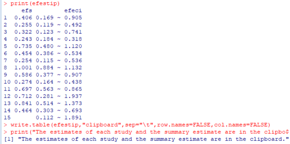
print(efestip)
write.table(efestip,"clipboard",sep="\t",row.names=FALSE,col.names=FALSE)
print("The estimates of each study and the summary estimate are in the clipboard.")
#############################################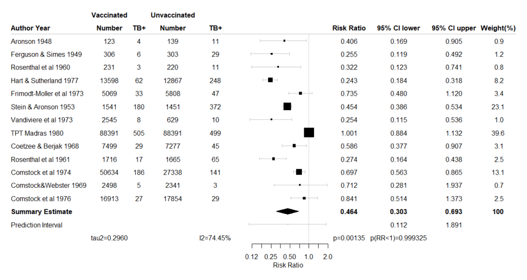
出力されたForest plotですが、確信区間だけでなく予測区間も出力します。Forest plotが出力された時点で各研究の効果推定値、95%確信区間、統合値とその95%確信区間、予測区間の値をコンソールに出力するとともに、クリップボードにコピーしますので、Excelの評価シートなどに結果の値を貼り付けることができます。
必要なパッケージがインストールされていない場合、以下のスクリプトを先に実行してください。未インストールのパッケージがインストールされます。metaforも含めました。また、RでStanを動かすためには、RToolsのインストールも必要になります。こちらから、Rのバージョンに合わせたバージョンのRToolsをダウンロードしてインストールしてください(430MB くらいある大きなプログラムです)。URL https://cran.r-project.org/bin/windows/Rtools/ 詳細は前の投稿を参照してください。
####Install packages for the first time####
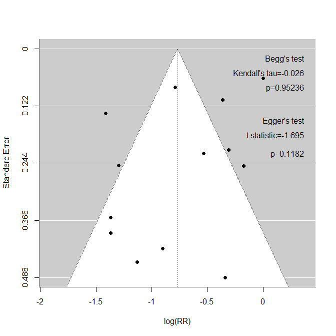
packneed=c("rstan","Rcpp","ggplot2","coda","dplyr","forestplot","bayesplot","HDInterval","metafor");current=installed.packages();addpack=setdiff(packneed,rownames(current));url="https://ftp.yz.yamagata-u.ac.jp/pub/cran/";if(length(addpack)>0){install.packages(addpack,repos=url)};if(length(addpack)==0){print("Already installed.")}Funnel plot作成のためのスクリプトを作成しました。Forest plotが出力された後に実行するとFunnel plotが出力されます。また、統計学的な非対称性の検定法である、Beggの検定、Eggerの検定も実行します。最後まで実行するとFunnel plot内にこれら検定の結果も書き出します。Funnel plotだけで十分な場合は、後半のAsymmetry test with Egger and Begg’s tests.の行以下のスクリプトは実行する必要がありません。また、Funnel plotは研究数が10(少なくとも5)件以上の場合に意味があるとされていますが、このスクリプトでは数による制限はしていませんの。
Funnel plot作成のためのスクリプト
########################
library(metafor)

#Plot funnel plot.
if(em == "RR"){
yi = log(rr)
vi=1/weights
sei = sqrt(1/weights)
mu = log(risk_ratio)
dev.new(width=7,height=7)
funnel(yi, sei = sei, level = c(95), refline = mu,xlab = "log(RR)", ylab = "Standard Error")
}

if(em == "OR"){
yi = log(or)
vi=1/weights
sei = sqrt(1/weights)
mu = log(odds_ratio)
dev.new(width=7,height=7)
funnel(yi, sei = sei, level = c(95), refline = mu,xlab = "log(OR)", ylab = "Standard Error")
}

if(em == "RD"){
yi = rd
vi=1/weights
sei = sqrt(1/weights)
mu = risk_difference
dev.new(width=7,height=7)
funnel(yi, sei = sei, level = c(95), refline = mu,xlab = "RD", ylab = "Standard Error")
}

#Asymmetry test with Egger and Begg's tests.
egger=regtest(yi, sei=sei,model="lm", ret.fit=FALSE)
begg=ranktest(yi, vi)

#Print the results to the console.
print("Egger's test:")
print(egger)
print("Begg's test")
print(begg)

#Add Begg and Egger to the plot.
fsfn=1
em=toString(exdat$label[6])
outyes=toString(exdat$label[4])
funmax=par("usr")[3]-par("usr")[4]
gyou=funmax/12
fxmax=par("usr")[2]-(par("usr")[2]-par("usr")[1])/40
text(fxmax,gyou*0.5,"Begg's test",pos=2,cex=fsfn)
kentau=toString(round(begg$tau,digits=3))
text(fxmax,gyou*1.2,paste("Kendall's tau=",kentau,sep=""),pos=2,cex=fsfn)
kenp=toString(round(begg$pval,digits=5))
text(fxmax,gyou*1.9,paste("p=",kenp,sep=""),pos=2,cex=fsfn)

text(fxmax,gyou*3.5,"Egger's test",pos=2,cex=fsfn)
tstat=toString(round(egger$zval,digits=3))
text(fxmax,gyou*4.2,paste("t statistic=",tstat,sep=""),pos=2,cex=fsfn)
tstap=toString(round(egger$pval,digits=5))
text(fxmax,gyou*5.1,paste("p=",tstap,sep=""),pos=2,cex=fsfn)
#####################################