
Google GeminiやOpenAIのGPTなどのAIを文献選定に使うツールを作成しているところですが、その精度と効率性をどう測るかについて知っておく必要があります。感度、特異度、適合率、F1スコア、WSSなどさまざまな指標について解説したスライドをGammaで作成しました。
カテゴリー: Systematic Review
A systematic review is a scientific investigation that focuses on a specific question and uses explicit, preplanned scientific methods to identify, select, assess, and summarize the findings of individual, relevant studies. It may or may not include a quantitative synthesis of the results from separate studies (meta-analysis).
Vibe CodingでRoB評価ツールを作成する
Vibe Coding というのは、プログラミング言語に則ってコードを入力してプログラムを作成するのではなく、プログラムの目的、機能や構成、変数、データ処理法、結果の表示法などを指定してAIにプログラミングさせることです。プログラム作成者は自分でプログラムを書く必要はありません。プログラミングの知識がある人ならスピーディーに効率的に様々なアプリケーションを作成することができます。
Google Gemini Proを使って Cochrane RoB2 for Cluster Randomized Trialsのガイダンスに従ったバイアスリスクの評価をするHTML-JavaScriptのツールを作成してみました。
ガイダンスのPDFファイルはこちらのサイトからダウンロードすることができます: URL https://sites.google.com/site/riskofbiastool/welcome/rob-2-0-tool/rob-2-for-cluster-randomized-trials
ダウンロードしたこのガイダンスのPDFファイルをGemini AIに読み込ませ、評価したい論文のPDFファイルをアップロードして評価させるという手順です。
標的論文のPDFは左側のパネルに画像として表示され、それぞれのドメインでAssessボタンをクリックして解析結果が表示されるようになっています。
URL https://stat.zanet.biz/sr/rob2-cluster.htm
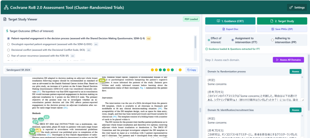
Target Studyを読み込ませる際に、測定されているアウトカムを抽出し、一覧を表示します。主要アウトカムは太字でmjrと言うマークが付き、副次アウトカムにはsecというマークが付きます。ラジオボタンで選択してAssess All Domainsボタンをクリックすると、自動でドメイン1から順次評価を進めることができます。右下にプログレスバーが表示されます。全体で4-5分で終了するはずです。
それぞれのドメインを個別に評価することもできます。その際は、一つのドメインが終わってから次のドメインの評価へと順番に進めていきます。その場合は、最後にサマリーの評価を行います。
結果はExport Docで、Docファイルとしてダウンロードすることができます。
上部に◯で表示される評価結果はCopyボタンで、数値データ(0, -1, -2)としてExcelシートに貼り付けられます。
論文の画像の中には、その根拠となる引用箇所にマークが付けられます。そのマークをクリックすると、判定とともに引用箇所の文章が表示されます。1ページごとに画像ファイルとして、後でまとめて記録のためにダウンロードして保存しておくことができます。
このツールを使うためにはGemini API Keyを設定する必要があります。Settings のメニューの中に Google AI Studio へのリンクがあるので、そこで API キーを発行してそれをコピーして貼り付けて使います。APIキーを設定したら、Usabel Gemini modelsをクリックし、モデル一覧からgemini-2.5-proを設定し、WebページのHTMLをダウンロードして保存し、以後はそのファイルを開いて使用します。APIキーは最初は無料枠で利用して、必要になったらTier 1の有料コースにアップグレードすればいいと思います。
引用文献のPMIDをPubMedを参照して調べる
論文の引用文献のフォーマットは様々で、PMIDとDOIが書かれていて、HTMLまたはPDFの場合はそれらにアクティブなリンクを設定してある場合もあります。PMIDが書かれていれば、それをPubMedで検索することで該当論文のAbstractを表示させることができますし、クリックするとその論文のAbstractを表示するURLのリンクを作成することもできます。
例えば、JAMAの論文のPDFをEdgeで開いて、引用文献の部分を1件だけコピーして貼り付けると以下の様になりました。JAMAのPDFの場合は、ジャーナル名以下のテキスト部分は青字でPubMedの該当論文へのリンクが設定されているので、その部分をクリックするとその論文のAbstractを表示することができます。PMIDが書かれていなくても、確認することができます。
- Nishihara R, Wu K, Lochhead P, et al. Long-term
colorectal-cancer incidence and mortality after
lower endoscopy. N Engl J Med. 2013;369(12):1095-
1105.
さて、引用文献にPMIDが書かれておらずリンクも設定されていない場合、あるいは印刷物の場合、どのようにしてそれを調べたらいいでしょうか?いくつかの方法が考えられます。
方法1:
マニュアルで、著者名3名+[au]、タイトルの語句3つ+[ti]、ジャーナル名+[ta]、年度[dp]をANDで結合してPubMedを検索する。
例えば、上記の文献であれば、nishihara[au] AND wu[au] AND lochhead[au] AND n engl j med[ta] AND 2013[dp]でPubMedを検索すると、PMID: 24047059の該当文献のAbstractを表示することができます。
ブラウザーのURLアドレスを書き込むフィールドにhttps://pubmed.ncbi.nlm.nih.gov/?term=nishihara[au] AND wu[au] AND lochhead[au] AND n engl j med[ta] AND 2013[dp]と書き込んでEnterキーを押しても該当文献のAbstractを表示することができます。つまり、https://pubmed.ncbi.nlm.nih.gov/?term=以降に検索式を書いてブラウザーで検索を実行させることで、PubMedが開かれ検索結果が表示されます。
方法2:
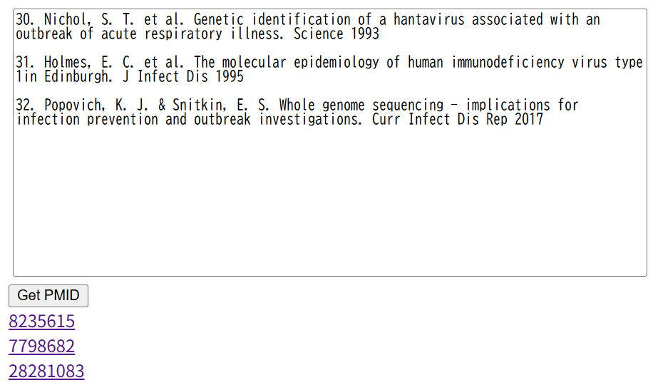
さらに、PubMedのE-utilitiesを利用することでもPMIDを得ることができますが、それを利用して検索式を作成し、PubMedからPMIDを得るウェブツールを作成してみました。PubMed PMID Searchと言います。URL: https://stat.zanet.biz/sr/get_pmid.htm
このウェブツールを使う方法ですが、書誌情報の内、著者名、タイトル、ジャーナル名、年度のデータを抽出して上記のように検索式を作成し、PubMedのE-utilitiesでPMIDの情報を引き出し、リンクを提示します。
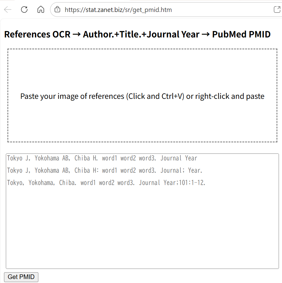
下のフィールドにサンプルのような形式で必要な情報を書き込んで、Get PMIDボタンをクリックするとボタンの下にPMIDがリンク付きで表示されます。著者名はコンマ区切りで、イニシャルを含めても含めなくてもよく、最後はピリオドで区切りを入れる;タイトルからできるだけ特徴的な語句を3つ程度スペースで並べ最後はピリオドで区切りを入れる;ジャーナル名はフルスペルでも短縮形でもいいがPubMedで用いられている形式で記述しスペースで区切って年度を続ける、というような形式で書き込みます。
上記のNishihara R 2013の例であれば、nishihara, wu, lochhead. colorectal cancer incidence. n engl j med 2013 と書き込んでGet PMIDをクリックするとリンク付きのPMIDがGet PMIDボタンの下に書き出されます。
また、以下の様なフォーマットの書誌情報でもOKです。
Dinubile MJ, Lupinacci RJ, Berman RS, Sable CA: Response and relapse rates of candidal esophagitis in HIV-infected patients treated with caspofungin. AIDS Res Hum Retroviruses 2002;18:903-8.
ジャーナルごとに様々なフォーマットが使われているので、今の所すべてに対応はできていませんが一か所を変えるだけで解読できる場合もあります。例えば、PubMedで一つの文献のAbstractを表示している状態で、Citeボタンから、AMAのフォーマットで文献情報をコピーできますが、このフォーマットの場合は、ジャーナル名の最後のピリオドを削除するだけで、解読できます。
複数の文献を参照したい場合は、各文献情報の最後に改行を2つ入れるようにしてください。
検索式に該当する文献が2つ以上ある場合、並べてPMIDが表示されるので、それらをクリックしてAbstractを表示して目的の文献を確認してください。
論文のPDFファイルの引用文献からテキストをコピーし上のフィールドに貼り付けて、形式を整えて、PMIDを得ることも可能です。
方法3:
画像として、文献情報をSnipping toolで取り込み、それを貼り付けて、OCRで文字情報に変換してからPMID情報を得る方法です。
たとえば、以下の文献情報は論文のPDFファイルの文献リストから得た画像です。
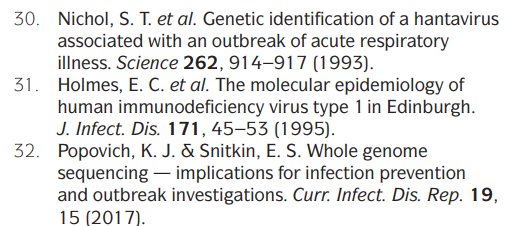
これをPubMed PMID Searchの上のフィールドをクリックして、Ctrl+Vで貼り付けます。あるいは、右クリックしてドロップダウンメニューから貼り付けを選んでも同じことができます。すると、上のフィールド内に画像がスケーリングされて表示され、すぐOCRで文字情報に変換され、下のフィールドに出力されます。OCRの精度は100%ではないので、マニュアルで修正が必要になることも多いです。
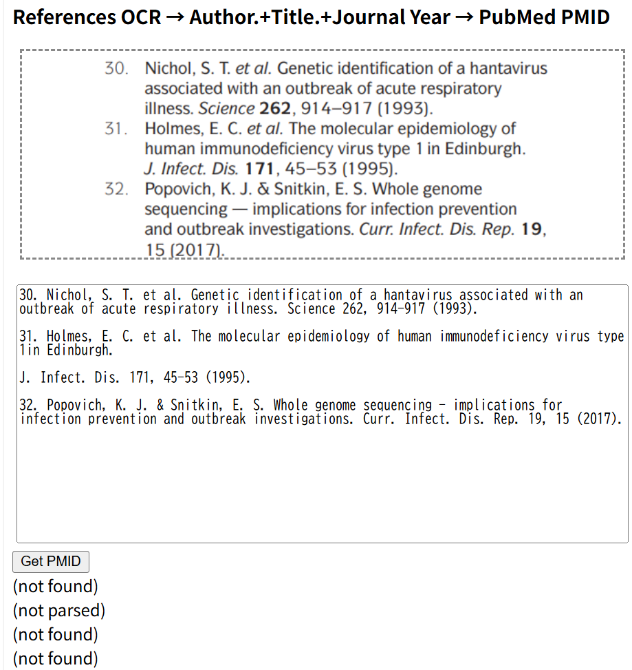
そのままでGet PMIDをクリックすると、この例ではnot foundあるいはnot parsedとなってしまいますので、マニュアルで少し修正します。ジャーナル名+スペース+年度にします。文献31はジャーナル名が改行されているので、これも修正し、ジャーナル名で短縮形にピリオドが使われているのも削除します。以下の図の様に修正したところ、3文献のPMIDが得られました。PMIDの部分をクリックすると各文献のAbstractをPubMedで表示することができます。
Get PMIDをクリックして、テキスト情報から検索式をうまく作れない場合は、not parsedと表示されます。PubMedを検索してもヒットしない場合はnot foundと表示されます。このような場合は、OCRで文字情報に変換する際に間違っている場合もありますし、ジャーナル名に今回の様にピリオドが入っているようなフォーマットの違いの場合などもあります。エラーを修正し、形式を整えれば、PMIDが得られるはずです。
以上文献情報からPMIDを調べる方法を紹介しました。
さて、PubMed PMID Searchは上のフィールドに文章を含む画像を貼り付けると、OCRで文字情報に変換しますが、英語と日本語に対応しています。OCRの機能はGoogleのTesseract.jsを利用しています。
頻度論派の信頼区間とベイズ統計の確信区間の違い
CochraneのRevMan, Rパッケージのmeta, metaforで用いられているメタアナリシスの手法は伝統的統計学すなわち頻度論派Frequentistの手法です。一方、ネットワークメタアナリシスのためのRパッケージであるgemtcはベイズ統計学に基づく手法を用いるベイジアンメタアナリシスを実行します。Arm-based modelを用いるネットワークメタアナリシスのためのRのパッケージであるpcnetmetaもベイジアンアプローチを用いています。ベイジアンアプローチでペアワイズのメタアナリシスをを行うには、OpenBUGS、JAGS、StanなどMarkov Chain Monte Carlo (MCMC)シミュレーションを実行するためのソフトウェアがRのパッケージであるR2OpenBUGS, rjags, rstanなどを介して用いられています。
頻度論派の手法で得られる統合値と信頼区間Confidence Intervalとベイジアンの手法で得られる統合値と確信区間(信用区間)Credible Intervalは同じように解釈すべきではありません。どのように違うのかを理解するために、以下メタアナリシスではありませんが、2群のイベント数からリスク比と信頼区間あるいは確信区間を計算する実例を示しながら解説したいと思います。
対照群のイベント割合(率)が0.5で介入群のイベント割合(率)が0.4が真のパラメータだとします。真のリスク比の値は0.4/0.5 = 0.8ですが、サンプルから得られる値は、必ずしも0.8にはなりません。例えば、対照群の症例数50例、介入群の症例数50例でランダム化比較試験が行われたとします。各群の50例中イベントが起きる人数は、ランダムサンプルであればこれらの値は二項分布に従い、必ず25人、20人になるというわけではありません。サンプリングの偶然の偏りで少しずつ違う値になります。そして、リスク比も必ず0.8になるわけではありません。これをRでシミュレートしてみます。
対照群の症例数をcsampleSize、イベント率をcprop、介入群の症例数をisampleSize、イベント率をipropで表すと、対照群のイベント数ceventsと介入群のランダムサンプリングで得られるイベント数ieventsをRでは次のスクリプトで得られます。
cevents <- rbinom(1, csampleSize, cprop) # 対照群イベント数 生成回数分
ievents <- rbinom(1, isampleSize, iprop) # 介入群イベント数 生成回数分
これは二項分布からランダムサンプルを得るrbinom()関数を用いていますが次のような考え方に基づいています。ランダム化比較試験の参加者が1名いた場合、その人が介入群に割り付けられると、0.5の確率でイベントが起きる訳ですが、結果として起きるか起きないかは0.5の確率です。次の対照群の参加者1名についても、同じことが言え、0.5の確率でイベントが起きる訳ですが、結果として起きるか起きないかは0.5の確率です。これを50人分繰り返した結果イベントが起きた人数は二項分布に従うので、Rのrbinom()関数では、rbinom(生成回数、ひとつの観測あたりの試行回数,各試行の成功確率)で試行回数でイベントが起きる回数=成功回数が得られます。通常は、同じランダム化比較試験は1回しか行わないので、生成する乱数の個数は1にした場合に相当しますが、この値を変数cycで設定すると、cycで設定した回数分のイベント数のデータが得られます。cycを例えば、100に設定すると、同じランダム化比較試験を100回行った場合の、対照群、介入群のイベント数をシミュレートすることができます。
cyc = 100; csampleSize = 50; cprop = 0.5
isampleSize = 50; iprop = 0.4
cevents <- rbinom(cyc, csampleSize, cprop) # 対照群イベント数 試行回数分
ievents <- rbinom(cyc, isampleSize, iprop) # 介入群イベント数 試行回数分
このスクリプトを実行すると、ceventsには25前後の値が、ieventsには20前後の値がそれぞれ100個格納されます。各群のイベント数からリスク比を計算することができるので、100個のリスク比の値を得ることができます。さらに、それぞれのイベント数と症例数から95%信頼区間を計算することができます。
リスク比の自然対数の95%信頼区間は以下の式で計算されます。すなわち、リスク比の自然対数の標準誤差 = 1/対照群のイベント数 + 1/介入群のイベント数 – 1/対照群の症例数 – 1/介入群のイベント数、をまず計算します。リスク比の自然対数に標準誤差×1.96をプラスマイナスし、計算結果のExponentialを求めると、リスク比の値に戻せます。なお、イベント数が0の場合はゼロの割り算が発生するので、0を0.5に置き換えておきます。
cevents[cevents == 0] = 0.5
ievents[ievents == 0] = 0.5
p_c <- cevents / csampleSize
p_i <- ievents / isampleSize
rr <- p_i / p_c
log_rr <- log(rr)
var_log_rr <- (1 / cevents + 1 / ievents) – (1 / csampleSize + 1 / isampleSize)
se_log_rr <- sqrt(var_log_rr) #Val(logRR)の標準誤差
z <- 1.96
lower_rr <- exp(log_rr – z * se_log_rr)
upper_rr <- exp(log_rr + z * se_log_rr)
グラフ表示までのすべてのスクリプトを以下に示します。変数の値を変えて様々な例をシミュレートすることができます。(スクリプトの一部は行頭に#を置いて実行されないようにコメント扱いにしています。プロット作成にggplot2パッケージを使っています。)
リスク比のシミュレーションのためのRスクリプト
###########################
#リスク比と95%信頼区間のシミュレーション

set.seed(123)
# パラメータ
cyc        <- 100      # 生成回数(同じ研究の回数)
csampleSize <- 50       # 対照群 50 人
isampleSize <- 50       # 介入群 50 人
cprop      <- 0.5		# 対照群イベント割合
iprop      <- 0.4		# 介入群イベント割合

# cyc回だけイベント数を生成 二項分布
cevents <- rbinom(cyc, csampleSize, cprop)  # 対照群イベント数 生成回数分
ievents <- rbinom(cyc, isampleSize, iprop)  # 介入群イベント数 生成回数分

cat("Control events:", cevents, "of", csampleSize, "\n")
cat("Intervention events:", ievents, "of", isampleSize, "\n")

# RR と 95%CI を計算できるかチェック
#if (cevents == 0 | ievents == 0) {
#  stop("どちらかの群でイベント数が0のため、この定義ではRRと95%CIを計算できません。")
#}
# ゼロイベントの場合の処理 0.5に設定する。
cevents[cevents == 0] = 0.5
ievents[ievents == 0] = 0.5
# リスク比
p_c <- cevents / csampleSize
p_i <- ievents / isampleSize
rr  <- p_i / p_c
log_rr <- log(rr)

# リスク比の自然対数の分散: Var(logRR) = (1/cevents + 1/ievents - 1/csampleSize - 1/isampleSize)
var_log_rr <- 1 / cevents + 1 / ievents - 1 / csampleSize - 1 / isampleSize
se_log_rr  <- sqrt(var_log_rr)		#Val(logRR)の標準誤差

# 95%信頼区間(logスケール → 元のスケール)
z <- 1.96
lower_rr <- exp(log_rr - z * se_log_rr)
upper_rr <- exp(log_rr + z * se_log_rr)

cat("RR =", rr, "\n")
cat("95% CI = (", lower_rr, ",", upper_rr, ")\n")

#######
library(ggplot2)

# 理論上のRR
true_rr <- iprop / cprop

# 結果をデータフレーム化
df <- data.frame(
  iter = 1:cyc,
  rr = rr,
  lower = lower_rr,
  upper = upper_rr
)

# true_rr が CI の外側にあるかどうかの判定
df$flag <- ifelse(true_rr < df$lower | true_rr > df$upper, "out", "in")

ggplot(df, aes(x = iter, y = rr)) +
  geom_point(aes(color = flag), size = 3) +
  geom_errorbar(aes(ymin = lower, ymax = upper), width = 0.1) +
  geom_hline(yintercept = true_rr, linetype = "dashed", color = "red") +
  coord_flip() +
  scale_color_manual(values = c("in" = "black", "out" = "red")) +
  labs(
    x = "Iteration",
    y = "Risk Ratio (RR)",
    title = "Risk Ratio with 95% CI (points outside true RR highlighted)"
  ) +
  theme_minimal(base_size = 14) +
  theme(legend.position = "none")


########
dev.new()
hist(rr, breaks = 30,
     main = "100 samples of RR",
     xlab = "RR",
     col = "lightblue",
     border = "white",
     freq = FALSE)   # 密度スケールにする

# 密度曲線を追加
#lines(density(rr),
#      col = "red",
#      lwd = 1)

###########################################################
上記のスクリプトを実行した結果です。点がリスク比の値で、バーは95%信頼区間を表します。
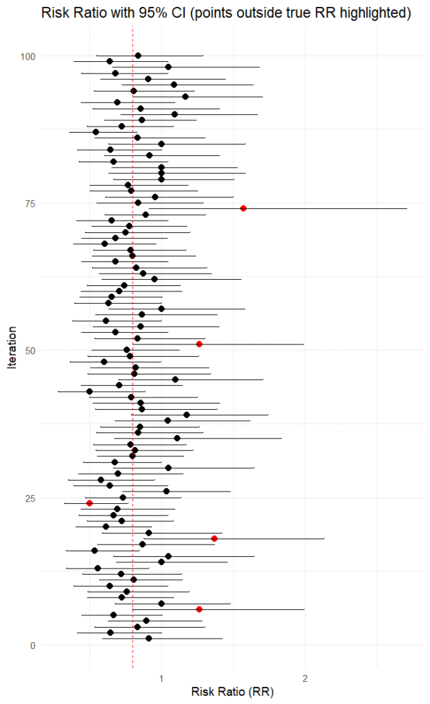
df$rr、df$lower、df$upperには生成回数分のリスク比、95%信頼区間の下限値、上限値、この例では100個の値が格納されていますので、例えば、df$rr[24], df$lower[24], df$upper[24]で24番目のリスク比、95%信頼区間の下限値、上限値の値が得られます。
1回のランダム化比較試験で得られるリスク比の値はこの値の中のどれか一つになります。ただし、もし、選択バイアスその他のバイアスの影響を受けると、リスク比の値は過大評価あるいは過少評価の方向へ少しずれますが、ここではバイアスは無いことを前提とします。ここで、たとえば、赤で示すリスク比の値が得られた場合、その95%信頼区間には真の値である0.8は含まれていません。今回のシミュレーションでは赤で示すリスク比は5個あり、100回中95回はその95%信頼区間に真の値が含まれていました。
頻度論派で得られる95%信頼区間は同じことを100回繰り返したら、95回は真の値を含んでいるという意味です。その時得られた信頼区間には真の値が含まれているか含まれていないかのどちらかです。95%信頼区間があたかも真の値の分布に基づいているという風に解釈するのは間違いです。リスク比の値も毎回異なりますが、信頼区間の値も毎回異なるので、それだけでも95%信頼区間があたかも真の値の分布に基づいているという風に解釈するのは間違いだということが分かります。
頻度論派で得られる95%信頼区間に基づいて、一定の閾値、例えば、リスク比1.0以上の確率を論じることはできません。今回のシミュレーションによる100個のリスク比の例を見てもわかる通り、リスク比1.0以上の確率は毎回異なります。信頼区間は真の値あるいはパラメータの分布に基づいているわけではありません。同じ試行を何回も繰り返し、そのたびに95%信頼区間を計算すると95%の場合は、真の値がその区間に含まれているという意味です。
上記の図を見ると、リスク比の値は真の値である、0.8の近くに多いことが分かります。リスク比の値のヒストグラムは以下の通りです。100個のサンプルですが、生成回数を多くするとより連続的なスムーズな確率密度分布が得られます。
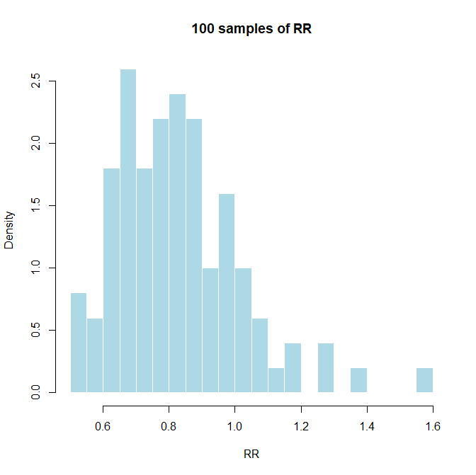
もし、真の値が分かっているのであれば、サンプルサイズとイベント数を指定することで、このような分布を知ることができます。
サンプルサイズが大きくなれば、真の値に近づくことができるということは言えますが、実際には有意であることを証明できるサンプルサイズでの1回の臨床試験の値しか知ることができないので、このようなパラメータの分布を頻度論派のアプローチでは知ることは困難です。
一方、ベイジアンのアプローチでは1回の試行の値を知ることで、それに基づいたパラメータの分布を知ることができます。パラメータは、ここではリスク比の真の値の分布と考えてもいいでしょう。そのパラメータの分布はそのデータに基づいていて、一定の閾値以上あるいは以下の、あるいはある範囲の確率をその時点で議論することが可能になります。もし、同じ研究をもう一度行った場合、それ以前のデータに基づく分布を事前分布として、その新しいデータでアップデートして事後分布を求めることができます。
Stanをrstanから動かして、対照群50例で25例にイベントが起き、介入群50例で20例にイベントが起きたというデータが得られた場合の、リスク比の事後分布を求めてみましょう。イベント率の事前分布はbeta(1, 1);ですが、区間[0, 1]上の一様分布です。従って、事前には有効性に関して全く情報がない状態です。Stan, rstanの使い方に関しては、以前の投稿を参照してください。
ベイジアンアプローチによるリスク比の推定:Stan, rstanを用いて
#Bayesian estimation of risk ratio with event rates in intervention group and comparator group.
library(rstan)
# data 例:対照群 25/50、介入群 20/50、リスク比0.8
sampleSize <- 50
cevents <- 25
ievents <- 20
stan_code <- "
data {
int<lower=0> N; // 各群のサンプルサイズ(同じ)
int<lower=0> y_c; // 対照群イベント数
int<lower=0> y_i; // 介入群イベント数
}
parameters {
real<lower=0, upper=1> p_c; // 対照群イベント率
real<lower=0, upper=1> p_i; // 介入群イベント率
}
model {
// 非情報事前 Beta(1,1)
p_c ~ beta(1, 1);
p_i ~ beta(1, 1);
// 尤度
y_c ~ binomial(N, p_c);
y_i ~ binomial(N, p_i);
}
generated quantities {
real rr;
real log_rr;
rr = p_i / p_c;
log_rr = log(rr);
}
"
# コンパイル
rstan_options(auto_write = TRUE)
options(mc.cores = parallel::detectCores())
bayes_rr_stan <- function(cevents, ievents, sampleSize,
iter = 50000, warmup = 25000, chains = 4) {
# Stan に渡すデータ
stan_data <- list(
N = sampleSize,
y_c = cevents,
y_i = ievents
)
# モデルをコンパイル
sm <- stan_model(model_code = stan_code)
# サンプリング
fit <- sampling(
sm,
data = stan_data,
iter = iter,
warmup = warmup,
chains = chains,
seed = 123
)
# 抽出
post <- rstan::extract(fit)
rr_samples <- post$rr
log_rr_samples <- post$log_rr
# 要約統計
rr_mean <- mean(rr_samples)
rr_median <- median(rr_samples)
ci_rr <- quantile(rr_samples, c(0.025, 0.975))
list(
fit = fit, # rstan オブジェクト(トレースプロット等に使える)
RR_mean = rr_mean,
RR_median = rr_median,
RR_CI95 = ci_rr,
RR_samples = rr_samples,
logRR_samples = log_rr_samples
)
}
# StanでMCMC実行
result <- bayes_rr_stan(cevents, ievents, sampleSize)
# 結果のコンソール出力
result$RR_mean
result$RR_median
result$RR_CI95
# 事後分布を可視化
#######Risk Ratio
hist(result$RR_samples, breaks = 50,
main = "Posterior of RR (Stan)",
xlab = "RR", col = "lightblue", border = "white")
dev.new()
hist(result$RR_samples, breaks = 50,
main = "Posterior of RR (Stan)",
xlab = "RR", col = "lightblue", border = "white",
freq = FALSE) # ★ 密度表示にするのが重要
# 密度曲線を追加
lines(density(result$RR_samples),
col = "red", lwd = 1)
text(1.5,1.5,paste("RR median =",round(result$RR_median,3)))
#######log Risk Ratio
dev.new()
hist(result$logRR_samples, breaks = 50,
main = "Posterior of RR (Stan)",
xlab = "RR", col = "lightblue", border = "white")
dev.new()
hist(result$logRR_samples, breaks = 50,
main = "Posterior of RR (Stan)",
xlab = "RR", col = "lightblue", border = "white",
freq = FALSE) # ★ 密度表示にするのが重要
# 密度曲線を追加
lines(density(result$logRR_samples),
col = "red", lwd = 1)
text(0.5,1.0,paste("log RR mean =",round(mean(result$logRR_samples),3)))
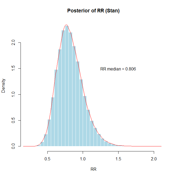
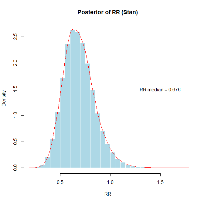
############################リスク比は以下の図の様になりました。iter = 50000, warmup = 25000, chains = 4なので、10万個の事後分布のサンプルです。リスク比の事後分布のサンプルの中央値0.8058、確信区間 0.5179~1.2334となりました。
自然対数に変換すると、左右対称の分布となり正規分布に近似します。
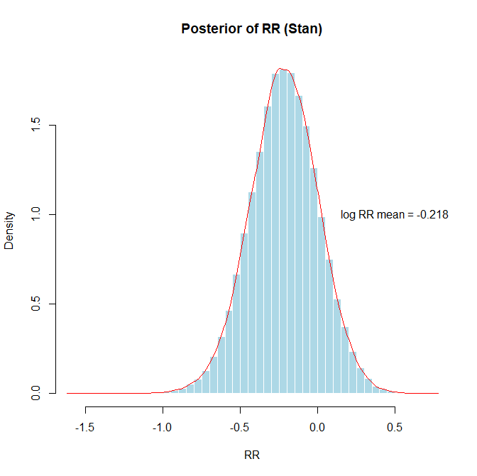
ベイジアンアプローチによるリスク比の分布でリスク比が1.0以上の確率は事後分布のサンプルから、mean(result$RR_samples >= 1.0)で求められます。0.15973でした。かなりの確率で介入群の方ででイベント数がより多くなることがあると考えられます。
もし、対照群では50例中27例、介入群では50例中18例でイベントが起きたというデータを得たとします。その場合のリスク比の値は0.6899 (95%CI 0.4259~1.0334)でグラフで示すと以下の通りです。このCIはCredible Intervalです。mean(result$RR_samples <= 0.8)でリスク比が0.8以下の確率を求めると0.78でした。
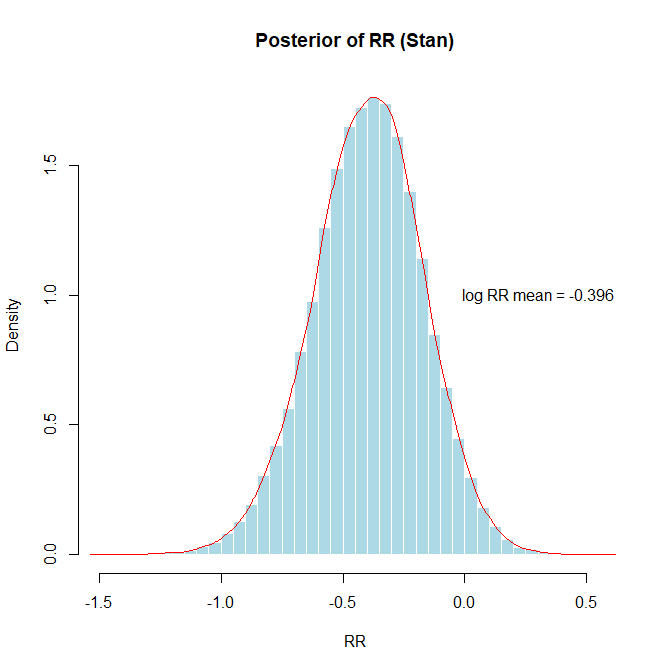
なお、自然対数に変換したグラフではlog RR mean = -0.396の描画の際text(0.3,1.0,paste(“log RR mean =”,round(mean(result$logRR_samples),3)))とx座標を少し左にずらしています。)
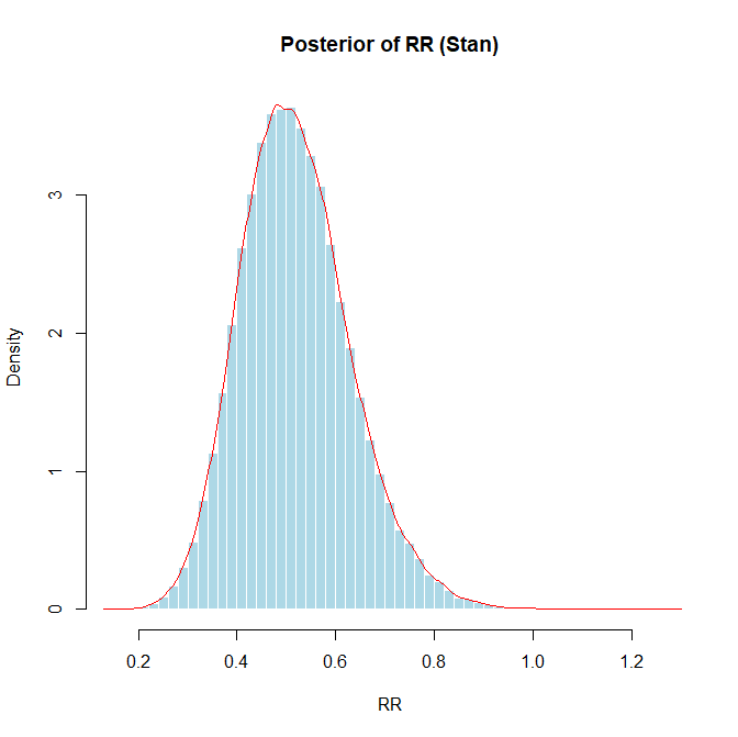
さらに、頻度論派アプローチで100個のリスク比をシミュレートした結果の内、95%信頼区間の範囲に真の値の0.8が含まれなかった例、対照群のイベント数34、介入群のイベント数17の場合のベイジアンアプローチでのリスク比を分析してみました。リスク比0.5192 (95%CI 0.3240~0.7603)となりました。リスク比が0.8以下の確率を求めると0.987でした。つまり、この95%確信区間には0.8の値は含まれないことが分かります。
メタアナリシスはほとんどの場合、頻度論派の手法が用いられていますが、統合値とその95%信頼区間の解釈で、ベイジアンアプローチの解釈の仕方をしないように注意する必要があります。
より分かりやすい解説をGamma.aiで作成してみました。こちらもご覧ください。
「頻度論派の信頼区間とベイズ統計の確信区間の違い」
以前作成したYouTubeの動画でも解説しています。
「信頼区間と確信区間の解釈:ベイジアンと頻度論派」