システマティックレビューでは採用文献あるいは除外文献の一覧を作成する必要があります。Cochraneレビューでは、そのような一覧は、Characteristics of studiesとCharacteristics of excluded studiesと呼ばれています。前者では、第一著者のFamily name 年度、Methods, Participants, Interventions, Outcomes, Identification, Notesが構成項目です。後者は第一著者のFamily name 年度と除外理由が提示されます。
また、MindsのSR用テンプレート(全体版 URL: https://minds.jcqhc.or.jp/methods/cpg-development/minds-manual/)では、【SR-3 二次スクリーニング後の一覧表】がそれに相当し、文献、研究デザイン、P、I、C、O、除外、コメントが構成項目です。こちらは、全文を読んで行う二次選定で除外された文献について、除外の項目で理由を記述するようになっていますので、一次選定で採用された文献については、すべてPICO要約を作成することになります。
論文のアブストラクトからPICOの要約とCommentsをAIで作成できるか試してみました。2025年11月19日の時点で、CopilotはSmart(GPT-5)を用い、GeminiはGemini PRO 2.5 FlashモデルはFastを用います。結論から言うと、ほぼそのまま使用できるレベルのPICO要約表が極めて短時間で作成できます。
PICO要約がAIで作成できれば、効率化が図れます。そこで、まず、アブストラクトを1つずつ処理するやり方を試してみます。PubMedでその文献のAbstractを提示させ、Abstractの部分を選択し、コピー操作を行って、以下のプロンプトの後に、貼り付けます。そして、Enter Keyを押すか、↑のボタン(Copilotの場合)あるいは⇨のボタン(Geminiの場合)をクリックします。書誌情報はここでは取り込まず、別の方法で抽出されている場合を想定しており、PICOとコメントだけです。
以下の論文のアブストラクトからPopulation, Intervention, Comparator, Outcome、すなわちPICOのそれぞれの要点およびコメントを書き出してください。PICOの要点は他の研究と比較する際にそれぞれの属性の違いが分かる程度に詳細を含めてください。Pの項には全症例数、Iの項には介入群の症例数、Cの項には対照群の症例数を入れてください。出力したテキストはコピーして貼り付けられるようにしてください。形式は以下の通りで、:から書き足して、各要素の最後は改行で区切ってください。研究デザインはランダム化比較試験はRCT、コホート研究はCohort、症例対照研究はCase-control、横断研究はCross-sectional、それ以外Othersに分類してください。LaTeXの数式環境($など)は用いずに、通常のテキストとして出力し、最後に改行が入る形式にしてください。
P: 対象者の要点。
I: 介入の要点。
C: 対照の要点。
O: アウトカムの要点。
Comments: 研究デザイン 研究全体に関するコメント。
****ここにAbstractのテキストを貼り付ける****
あっという間に、以下のようなPICO要約が出力されます。この例の文献は最後に引用を付けています。
| P: 138例がランダム化され、123例が解析対象。対象は肝硬変を伴う肝細胞癌患者。背景はChild-Pugh Aが70%、アルコール性肝硬変76%、Okuda stage Iが71%、多結節型腫瘍70%、門脈枝血栓10%。 I: 62例。Transarterial Lipiodol Chemoembolisation (TACE)+Tamoxifen併用療法。 C: 61例。Tamoxifen単独療法。 O: 主要アウトカムは全生存率とQOL(Spitzer Index)。2年生存率はTamoxifen群22%、TACE群25%(P=0.68)。QOLに有意差なし(P=0.70)。サブ解析(Okuda I)では2年生存率Tamoxifen群28%、TACE群32%(P=0.58)。予後因子としてAFP>400ng/mL、腹痛、肝腫大、Child-Pughスコアが有意。 Comments: RCT。多施設第III相試験。TACE+TamoxifenはTamoxifen単独と比較して生存率・QOLの改善を示さず、予後因子の解析が主な意義。 |
もう少し簡略化したPICO要約のためのプロンプトが以下のプロンプトです。
以下の論文のアブストラクトからPopulation, Intervention, Comparator, Outcome、すなわちPICOのそれぞれの要点およびコメントを書き出してください。出力したテキストはコピーして貼り付けられるようにしてください。形式は以下の通りで、:から書き足して、各要素の最後は改行で区切ってください。研究デザインはランダム化比較試験はRCT、コホート研究はCohort、症例対照研究はCase-control、横断研究はCross-sectional、それ以外Othersに分類してください。LaTeXの数式環境($など)は用いず、**も不要です。通常のテキストとして出力し、最後に改行が入る形式にしてください。
P: 対象者の要点。
I: 介入の要点。
C: 対照の要点。
O: アウトカムの要点。
Comments: 研究デザイン 研究全体に関するコメント。
****ここにAbstractのテキストを貼り付ける****
その出力結果です。だいぶ短くなりました。”Pの項には全症例数、Iの項には介入群の症例数、Cの項には対照群の症例数を入れてください。”を入れた方がいいかもしれません。
| P: 肝硬変を伴う肝細胞癌患者。対象は1995~2002年に登録された患者138例のうち123例が解析対象。主な背景はChild-Pugh Aが70%、アルコール性肝硬変が76%、Okuda stage Iが71%、多結節型腫瘍が70%、門脈枝血栓が10%。 I: トランス動脈性リピオドール化学塞栓療法(TACE)+タモキシフェン併用。 C: タモキシフェン単独。 O: 全生存率(2年生存率:TACE群25%、タモキシフェン群22%、有意差なし)、QOL(Spitzer Indexで両群差なし)。サブ解析ではOkuda stage I群でも有意差なし。予後因子としてAFP高値、腹痛、肝腫大、Child-Pughスコアが独立因子。 Comments: RCT 多施設共同第III相ランダム化比較試験。TACE併用は生存率・QOLの改善を示さず、予後因子の探索的解析が主な意義。。 |
Geminiでも同じような結果が得られますが、以下の様になります。
| P: 肝細胞癌(HCC)および肝硬変を有する患者。全症例数138名(適格症例123名)。Child-Pugh分類Aが70%、アルコール性肝硬変が76%、OkudaステージIが71%、多結節性腫瘍が70%、区域性門脈血栓症が10%。 I: 経動脈的リピオドール塞栓術(TACE)とタモキシフェンの併用。介入群の症例数62名(適格症例)。 C: タモキシフェン単独療法。対照群の症例数61名(適格症例)。 O: 全生存期間(2年時点の生存率がタモキシフェン群22% vs TACE群25%でP=.68)。生活の質(Spitzer Index)。 Comments: 研究デザイン: RCT。研究全体に関するコメント: HCCと肝硬変の患者に対する緩和的治療において、TACEとタモキシフェンの併用はタモキシフェン単独と比較して、生存期間も生活の質も改善しないことが示唆された。AFP > 400 ng/mL、腹痛、肝腫大、Child-Pughスコアが独立した予後因子として同定された。OkudaステージIのサブグループ解析でも有意な生存期間の改善は認められなかった。 |
簡略版
| P: 肝細胞癌(HCC)および肝硬変を有する患者。 I: 肝動脈塞栓化学療法(TACE)とタモキシフェンの併用療法。 C: タモキシフェン単独療法。 O: 全生存期間(overall survival)、および生活の質(quality of life, Spitzer Index level)。 Comments: 研究デザイン: RCT 研究全体に関するコメント: 多施設共同の第III相ランダム化比較試験で、肝細胞癌に対するTACEとタモキシフェンの併用療法の有効性をタモキシフェン単独療法と比較しています。結果は、TACEの追加が生存期間も生活の質も改善しないことを示唆しています。 |
続けて、別のアブストラクトの処理をさせたい場合は、「同じように処理して。」のプロンプトに続けてアブストラクトを貼り付けて実行させるだけで大丈夫です。
プロンプトは必要に応じて、修正、追加していろいろ試してみて下さい。今回も自分で考案したさまざまなプロンプトを試してみましたが、一応使用可能だと思ったので、紹介しました。
さらに、複数の文献のPICO要約表の作成も可能です。例えば、PubMedでPMIDのリストを作成するなどして、必要な文献の検索結果を表示させます。それをAbstract形式でSaveしてテキストファイルとしてダウンロードします。他の方法で作成する場合も、書誌情報とアブストラクトが含まれている必要があります。
そして、そのテキストファイルをCopilotのチャットエリア(プロンプトを書き込むフィールド)にドラグアンドドロップします。(Geminiも同じです)。それに続けて、以下のプロンプトを書き出して、Enter Keyを押すと結果が得られます。なお、チャットエリアで、改行を入れたい場合は、Shift Keyを押しながら、Enter Keyを押します。途中で間違ってEnter Keyを押してしまうと、そこでAIの応答が始まってしまうので、注意が必要です。
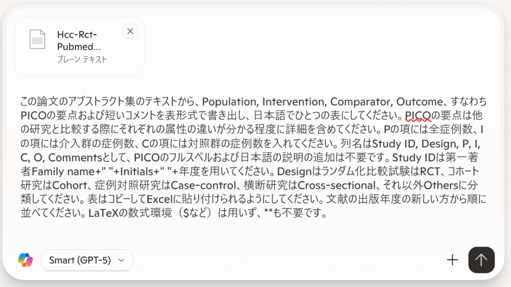
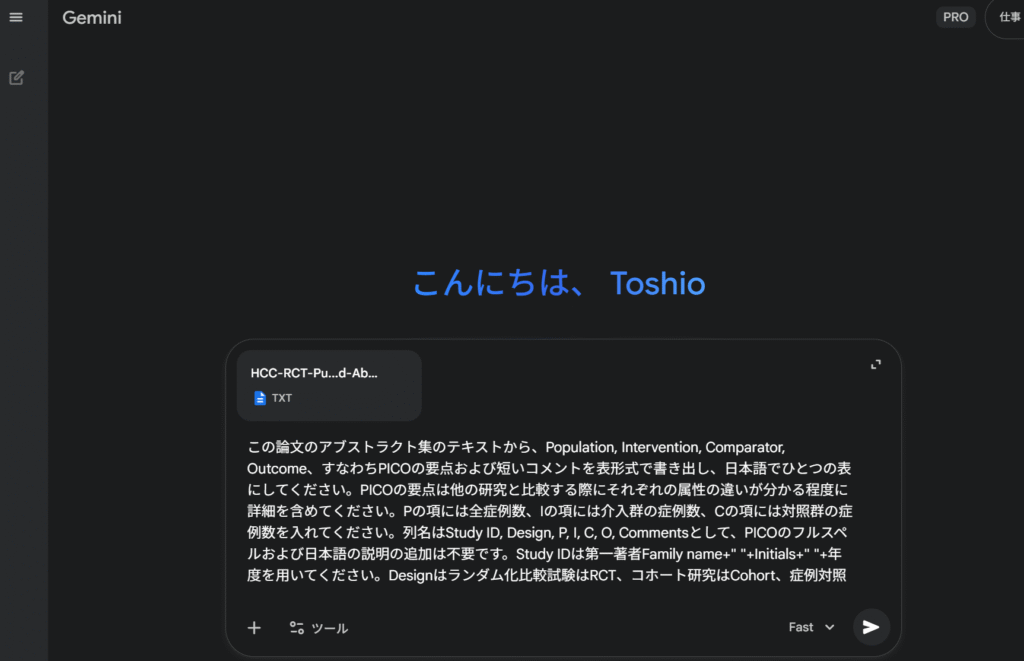
この論文のアブストラクト集のテキストから、Population, Intervention, Comparator, Outcome、すなわちPICOの要点および短いコメントを表形式で書き出し、日本語でひとつの表にしてください。PICOの要点は他の研究と比較する際にそれぞれの属性の違いが分かる程度に詳細を含めてください。Pの項には全症例数、Iの項には介入群の症例数、Cの項には対照群の症例数を入れてください。列名はStudy ID, Design, P, I, C, O, Commentsとして、PICOのフルスペルおよび日本語の説明の追加は不要です。Study IDは第一著者Family name+" "+Initials+" "+年度を用いてください。Designはランダム化比較試験はRCT、コホート研究はCohort、症例対照研究はCase-control、横断研究はCross-sectional、それ以外Othersに分類してください。表はコピーしてExcelに貼り付けられるようにしてください。文献の出版年度の新しい方から順に並べてください。LaTeXの数式環境($など)は用いず、**も不要です。簡略版
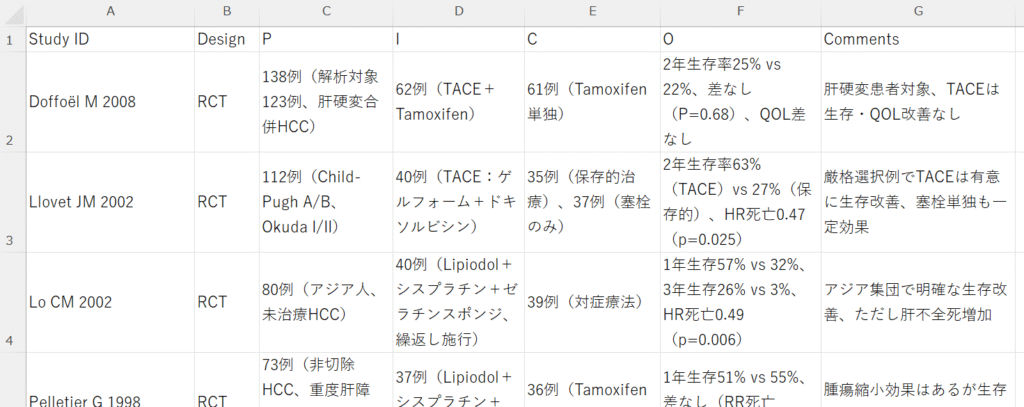
この論文のアブストラクト集のテキストから、Population, Intervention, Comparator, Outcome、すなわちPICOの要点および短いコメントを表形式で書き出し、日本語でひとつの表にしてください。Pの項には全症例数、Iの項には介入群の症例数、Cの項には対照群の症例数を入れてください。列名はStudy ID, Design, P, I, C, O, Commentsとして、PICOのフルスペルおよび日本語の説明の追加は不要です。Study IDは第一著者Family name+" "+Initials+" "+年度を用いてください。Designはランダム化比較試験はRCT、コホート研究はCohort、症例対照研究はCase-control、横断研究はCross-sectional、それ以外Othersに分類してください。表はコピーしてExcelに貼り付けられるようにしてください。文献の出版年度の新しい方から順に並べてください。LaTeXの数式環境($など)は用いず、**も不要です。Copilotでは直接Excelファイルとして保存することもできますが、結果のコピーボタンをクリックして、Excelシートに貼り付け、不要な部分を削除する方法がスピーディーです。以下の例は、簡略版ではない方のプロンプトの結果です。
GeminiではGoogleドライブのスプレッドシートへ直接出力できるボタンが出てきます。Googleスプレッドシートから、Excelファイルとして保存することができます。
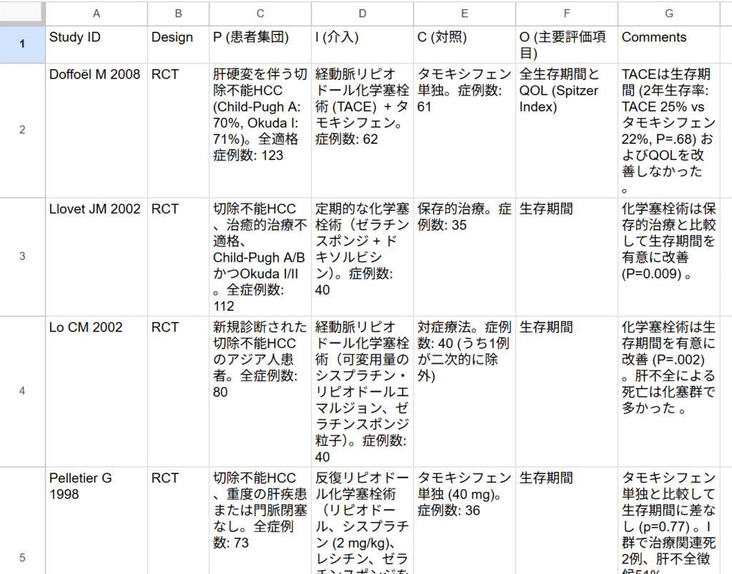
これらの表を自分で入力することを考えると、極めて効率化が図れると言えます。今回の例では6文献でしたが、本当にあっという間にできてしまいます。除外の列は入れてありませんが、Excel間のコピー・貼り付けで、【SR-3 二次スクリーニング後の一覧表】はあっという間に作成できそうです。
また、列名がプロンプトの指示通りにならなかったり、その他にも意図したとおりにならないことがあり得ますので、そのような際にはプロンプトを追加するなり、工夫してみて下さい。
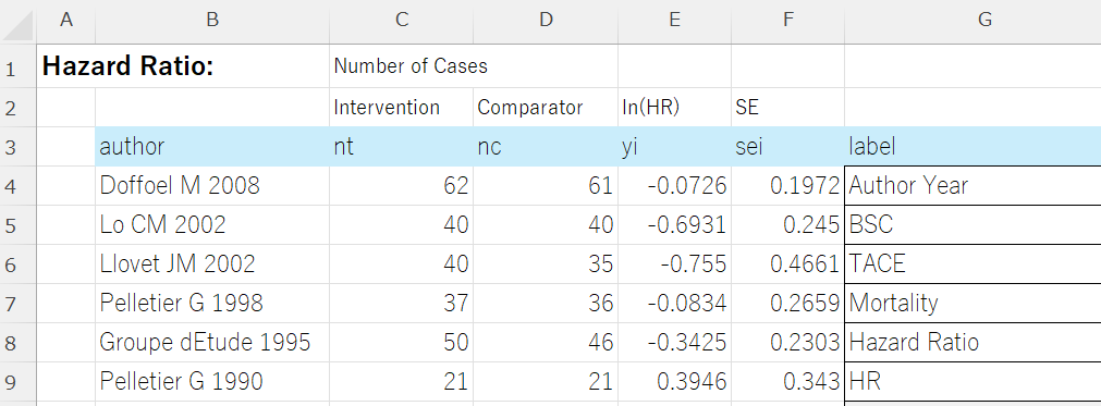
PubMedでAbstract形式でSaveしたテキストファイルだけでなく、必要な情報を含むExcelファイルからも同じことができます。CopilotもGeminiもExcelファイルをドラグアンドドロップで受け付けてくれますので、上記のテキストファイルと同じように読み込ませることができます。例えば、次のようなExcelファイルを文献処理用のソフトウェアで用意して、使うことができます。
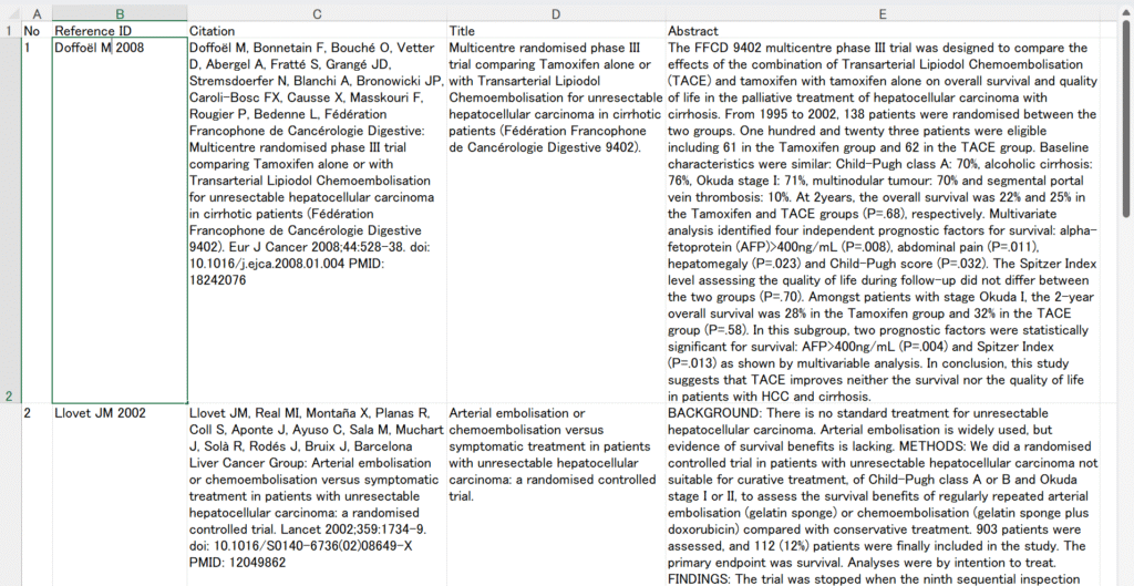
この例の場合、プロンプトのStudy IDの取り込みに関する部分を、”Study IDは第一著者Family name+” “+Initials+” “+年度を用いてください。”から”Study IDはReference IDの値をそのまま用いてください。”に書き換えてもいいでしょう。
またBunkanという文献管理用のマクロが付いたExcel Bookを使う場合、まずファイルを編集可能にするために、ファイルのアイコンを右クリックして、プロパティを選択し、全般のタブの画面で下の方のセキュリティの項目の許可するにチェックを入れ、OKボタンをクリックします。これでコピー操作ができるようになるので、目的のSheetの下の方にあるラベルを右クリックして、ポップアップメニューから移動またはコピーを選択し、左下のコピーを作成するにチェックを入れ、移動先ブック名で(新しいブック)を選択し、OKをクリックします。これで、新しいExcelファイルに同じ文献一覧が表示されますので、そのファイルをファイル名を付けて、xlsxファイルとして保存します。このようにして保存したExcelファイルはCopilotあるいはGeminiにドラグアンドドロップして読み込ませることができますので、あとは同じように処理できます。
さて、最後に研究デザインの分類については、すべてのデザインについてテストをしていないので、もしうまく分類されなかった場合、その部分のプロンプトを書き換える必要があるかもしれません。また、今回はアブストラクトの情報からPICO要約を作成しましたが、Copilot、GeminiはPDFファイルもドラグアンドドロップで情報を読み込ませることができるので、ひとつずつであれば全文のPDFファイルからもPICO要約ができるかもしれません。全文に合わせてプロンプトの修正が必要な箇所が出てくるかもしれませんが。
また、PICO要約は一次選定後の文献一覧から作成しますが、一次選定もAIにやらせることもできます。適格基準:採用基準と除外基準をプロンプトで記述して、それで選定された文献からPICO要約を作成するようにプロンプトを記述すれば1ステップで実行できるはずです。ただし、まだ本格的には試していなので、文献数を制限する必要があるかもしれませんし、ASReviewなどの機械学習を用いる方法と比較することも必要になるでしょう。(ASReviewに関する以前の投稿はこちら)。
文献:
最初の例の論文:Doffoël M, Bonnetain F, Bouché O, Vetter D, Abergel A, Fratté S, Grangé JD, Stremsdoerfer N, Blanchi A, Bronowicki JP, Caroli-Bosc FX, Causse X, Masskouri F, Rougier P, Bedenne L; Fédération Francophone de Cancérologie Digestive. Multicentre randomised phase III trial comparing Tamoxifen alone or with Transarterial Lipiodol Chemoembolisation for unresectable hepatocellular carcinoma in cirrhotic patients (Fédération Francophone de Cancérologie Digestive 9402). Eur J Cancer. 2008 Mar;44(4):528-38. doi: 10.1016/j.ejca.2008.01.004. Epub 2008 Jan 31. PMID: 18242076.