NotebookLMの使用法概要
NotebookLM(以下NLM)はArtificial Intelligence (AI)が参照する情報ソースを利用者が設定できるのが特徴である。ウェブで参照できる情報に基づいて回答を生成するわけではない。ソースとして設定できる情報は様々で、ウェブ上の情報は特定のURLをソースにアップロードすることで、そのページの情報をソースとして利用でき、それだけでなく、PDFファイル、テキストファイル、YouTube動画などさまざまな情報ファイルをソースとして利用することができる。
アップロードがサポートされているファイル形式は、PDF, .txt, Markdown, 音声(例: mp3), .docx, .avif, .bmp, .gif, .ico, .jp2, .png, .webp, .tif, .tiff, .heic, .heif, .jpeg, .jpg, .jpeである。さらに、Googleドライブのファイルや、コピーしたテキストを貼り付けて利用することもできる。
NLMのサイト(https://notebooklm.google.com/ )を開き、右上の+新規作成ボタンをクリックすると、最初にソースをアップロードするパネルが表示される。
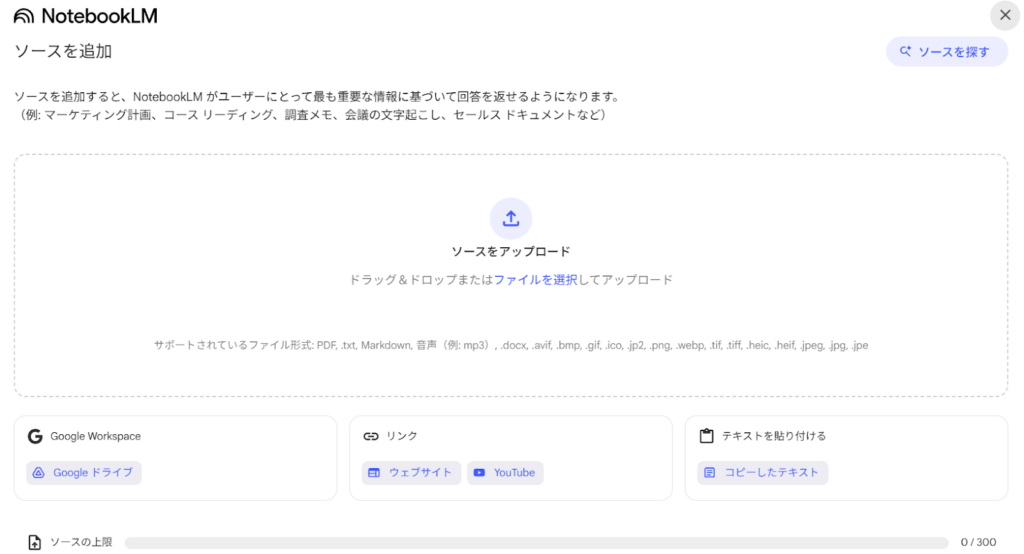
複数のファイルをまとめてドラッグアンドドロップして、アップロードすることができる。アップロードが完了するとそれらの概要が表示される。(概要の表示には時間がかかる場合もある)。新規にノートを作成した場合、ノートのタイトルはソース情報から自動的に作成されるが、必要に応じて書き換える。
左のソースのパネルに、ソースの情報が表示される。ソースを追加したい場合は、左のソースのパネルの上にある+ソースを追加のボタンをクリックして、ソースアップロードのパネルが表示させることができる。
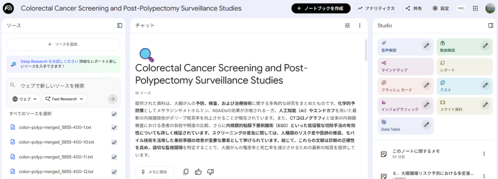
NLMの画面は、ソース、チャット、Studioの3つのパネルからなる。Studioのパネルには、音声解説、動画解説、マインドマップ、レポート、フラッシュカード、テスト、インフォグラフィック、スライド資料、Data Tableの作成のためのボタンが並んでいる。その下に、保存したメモの一覧が表示される。
中央のチャットのパネルの下に、プロンプトを書き込むフィールドがあり、書き込んでからEnterキーを押すか、→ボタンをクリックすると回答が生成され、それをメモとして保存することができる。
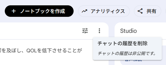
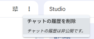
チャットのパネルの上には、点が縦に3つ並んだボタンがあるが、そこをクリックして、チャットの履歴を削除を選択するとチャットの履歴を削除できる。NLMは連続していくつかのプロンプトを実行した場合、前のプロンプト実行の情報が残っており、それを前提としてプロンプトが実行されるため、それらの履歴をクリアして新規にプロンプトを実行する必要がある場合は、一度チャットの履歴を削除する必要がある。
左のソースのパネルには、アップロードしたファイル名、URLなどの一覧が表示され、ソースの種類によって違うアイコンが用いられている。また、プロンプトを実行する際には、ソースとして使用したいものだけをチェックを入れることで、目的に合わせた選択ができる。ソースの一覧の一番上が、すべてのソースを選択になっており、このチェックボックスですべてを選択したり、はずしたりができる。
また、ソース名を指定して、2つのPDFファイルの内容を比較させたりすることもできる。例えば、作成マニュアルのPDFファイルをアップロードしておき、それに従って作成した文書をアップロードしてある場合、その内容がマニュアルに従っているかをチェックさせるような作業も可能である。
また、プロンプトで得られた回答をメモに保存したら、Studioのパネルに表示されているメモのタイトルから、それを開くと下の方に、ボタンがあり、ソースに変換することができる。そのソースだけを選択して、インフォグラフィックを作成したり、動画解説を作成したりすることもできる。
医学知識のアップデート
特定のテーマについて医学知識をアップデートしたい場合、さまざまな方法が考えられるが、PubMedから論文のアブストラクトの情報を収集し、それらをNLMのソースにアップロードして、プロンプトで必要な情報を引き出すことができるか試してみることにする。元の情報は英語であっても、プロンプトは日本語で書くことができ、回答も日本語で得られる点は利点の一つである。
NLMのAI機能を利用することで、例えば、数千件という多数の論文のアブストラクト情報に基づいて、必要な情報を引き出すことが可能になると考えられ、文献の選定、読み込みの作業をすることなく、知りたい情報を得ることができるかもしれない。また、PICO形式のクエスチョンに対する回答を得たい場合、システマチックレビュー/メタアナリシス、ランダム化比較試験(randomized controlled trial, RCT)に限定して文献検索を行った場合の、文献選定の過程を省略できることも考えられる。さらに、PICO形式に限定されることなくさまざまな疑問に回答を得られることが可能になると考えられる。
ただし、AIの限界がどこに現れるか予測できない点もあり、結果をそのまますべて正しいものとして受け止めない注意が必要である。
医学文献の収集
PubMedでは、ほとんどの文献はアブストラクトまでは入手することができる。著者、タイトル、アブストラクトの情報を多数の文献から収集して、それらをソースとして、NLMにアップロードする。目的すなわち知りたいことに対して、偏りなく、網羅的に文献を収集することが重要になる。
操作手順
1.知りたいことを明確にする。
いわゆるForground questionでPICO形式のクエスチョン、例えば、「大腸ポリペクトミーを受けた患者で1年後に大腸鏡によるフォローアップ検査を受けると3年後に検査を受ける場合と比べて大腸癌の発症が減少するか?」
いわゆるBackground question「大腸ポリープ治療後のサーベイランスはどのようにすべきか?」の様な、5W1Hタイプのクエスチョン。*What, Who, When, Where, Why, How
いずれの場合も、以下の項目は明確に定義する必要があるであろう。
対象者:疾患、病態、他
介入、診断法、検査、リスクファクターなど
疾患のアウトカム、介入の効果を分析するために測定されるアウトカム(アウトカムの内容)、診断のアウトカムとしての疾患・病態、診断精度など
2.知りたいこと/クエスチョンに回答を与えるであろう研究=標的研究はどのようなものかを熟慮する。
研究デザイン
特定の研究デザインに限定した方がいい場合、例えば、特定の治療に関して知りたい場合であれば、文献検索の段階で、診療ガイドライン、メタアナリシス/システマティックレビュー、ランダム化比較試験に限定する方法をとることもできる。
3.標的研究のタイトル、アブストラクト、統制語に含まれると思われる語句を明確にする。
Text word (TW)
同義語 Thesaurus
MeSH (MH)、Entry word → MeSH databaseの参照が必須
4.準備的文献検索を実施し、用いるべき検索語句やMeSH termsを確認する。
meta-analysis[TA]やrandomized controlled trial[PT]、必要な場合年度 (例:2022:2025[dp]) をANDで組み合わせ少数の文献を引き出す。
標的文献に近い文献を見つけ、Abstractを表示させ、MeSH termsを表示させて、標的文献に必須の用語をMeSH databaseで開いて、階層構造を確認し、関連した語句を調べる。
既知の文献がある場合、その文献をPubMedで検索して、アブストラクトを表示させ、MeSH termsを確認する。
5.目的に応じて研究デザインを限定する検索フィルターを決める。
NLMを用いる場合、大量の情報を扱えるので、文献選定作業を考慮して、文献数を少なくすることを考える必要はない。目的に応じて、情報ソースに偏りがなく十分な情報が得られるように考える。
clinical trial[PT] OR meta-analysis[PT] OR practice guideline[PT] OR systematic[sb]
clinical trial[PT]にはrandomized cotnrolled trial[PTとcontrolled clinical trial[PT]は下位概念に含まれる。
RCTに限定する場合:randomized cotrolled trial[PT]
Cochrane RCT filter 感度最大化:(randomized controlled trial [pt] OR controlled clinical trial [pt] OR randomized [tiab] OR placebo [tiab] OR drug therapy [sh] OR randomly [tiab] OR trial [tiab] OR groups [tiab])
Cochrane RCT filter 感度・特異度最大化:(randomized controlled trial [pt] OR controlled clinical trial [pt] OR randomized [tiab] OR placebo [tiab] OR clinical trials as topic [MeSH:noexp] OR randomly [tiab] OR trial [ti] NOT(animals [mh] NOT humans [mh]))
言語、人対象: humans[mh] AND (english[la] OR japanese[la])
アブストラクト有り: hasabstract[tw] *アブストラクト有りに限定する。
5.検索式を構成しPubMed検索を実施する。
検索式の作成、PubMed検索にはpmSearch(https://stat.zanet.biz/sr/pmsearch.htm)を利用すると便利である。論理演算子 OR、AND、NOT。ただし、NOTは原則使用しない。
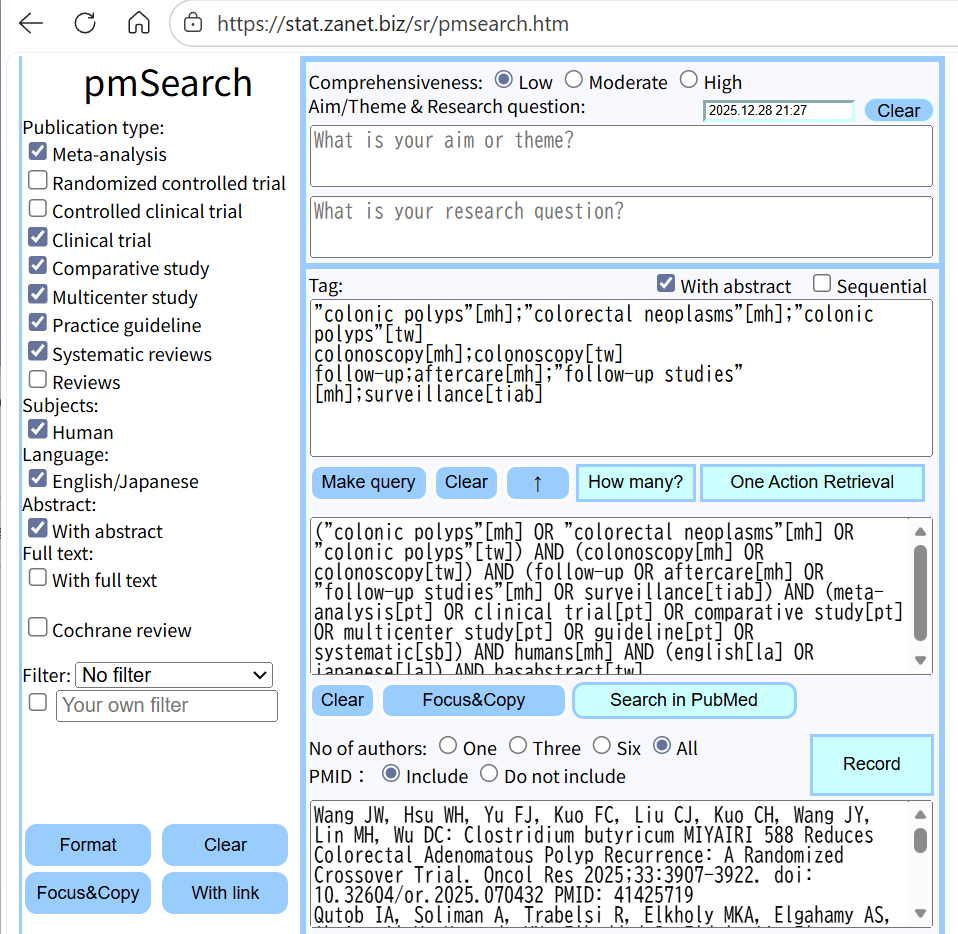
上から3段目のフィールドに検索語句を書き込むと、その下のフィールドに検索式が自動で作成される。ORは;を用いる。改行はANDとして扱う。
治療的介入がテーマの場合であれば、少なくとも、CochraneのRCTフィルターのいずれかを組み合わせた検索式とPubMedのPublication typeのいくつかを組み合わせた検索式の2種類を用いるようにする。左のパネルにある、Publication typeにチェックを入れて、さらにFilterからCochraneのRCT用フィルターなどを選択して組み合わせることができる。また、Population、Intervention (PI)の語句だけで検索し、結果が数千件程度であれば、Humanに限定するだけでも十分であろう。
様々な検索式を試す場合、How many?で一度文献数を確認する。
Search in PubMedをクリックするとPubMedが開かれて、その検索式で検索が実行される。さらに、MeSH termsの検討をすることも考える。また、スペルのミスなどが見つかる場合もある。
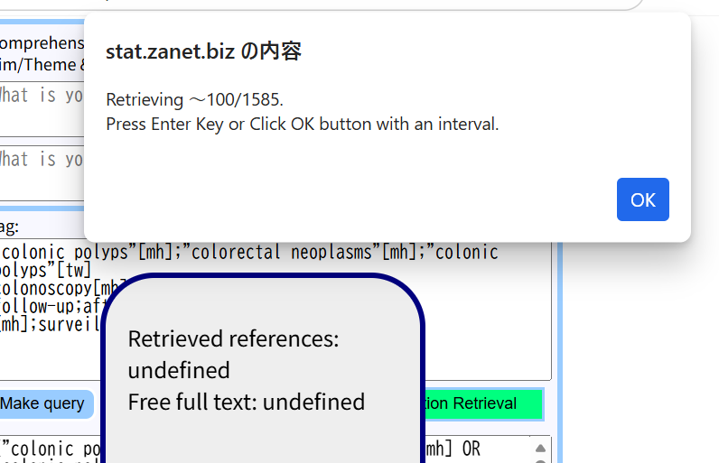
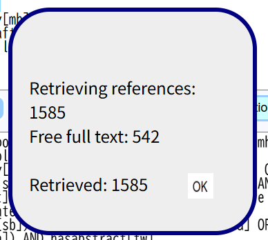
検索式が確定したら、上の図の様に、With abstractにチェックを入れて、One Action Retrievalをクリックすると、100件ずつEnterキーを押しながら(あるいはOKボタンをクリックしながら)、PubMedから、検索式に適合する文献がダウンロードされる。
終了すると、下のフィールドに結果が書き込まれ、アブストラクトを含む文献一覧表が別のタブで表示される。
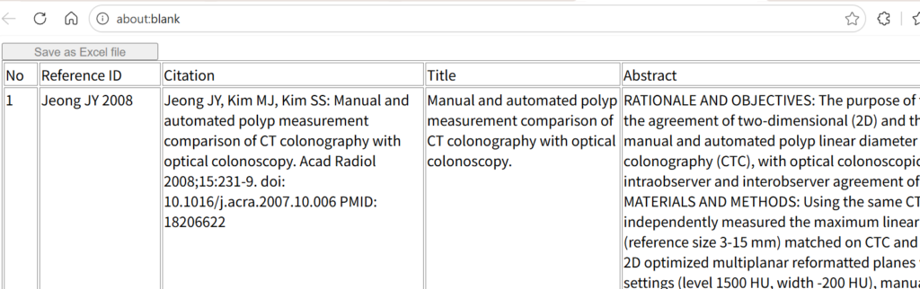
アブストラクトを含む文献一覧表の上にある、Save as Excel fileのボタンをShiftキーを押しながらクリックすると、結果をテキストファイルとして保存できる。保存したファイルを後で、400件ずつのテキストファイルに分割して、NLMのソースにアップロードするのに用いる。
pmSearchのウインドウに戻り、引き出された文献数を確認しながら、OKボタンをクリックする。
一番下のフィールドに検索結果の文献一覧が含まれているので、その左のWith linkボタンをクリックすると文献一覧の表が新しいタブに表示される。(Recordボタンをクリックしても文献の一覧表を作成できるが、文献数が約1000件を超えると処理に時間がかかるため、今回の目的には用いない。)
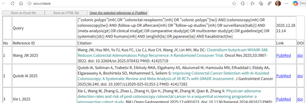
検索式と検索日時が1行目に記録されているので、左上にあるSave as HTML fileをクリックしてファイル名を付けて保存しておく。あとで、保存ファイルをダブルクリックするとブラウザで開いてみることができる。また、LinkのPubMedの部分をクリックするとその文献のAbstractをPubMedで開いてみることができる。
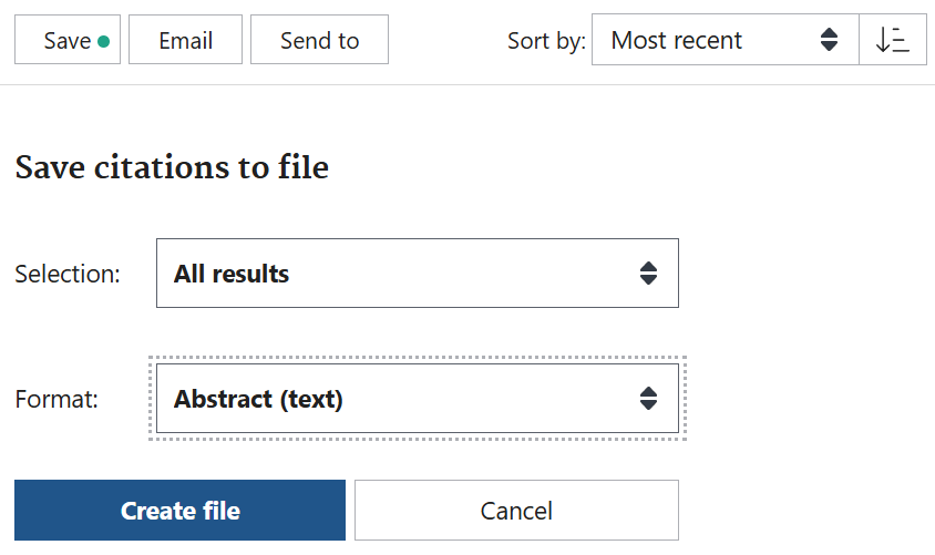
また、pmSearchでSearch in PubMedをクリックすることでPubMedで検索結果を表示し、アブストラクトを含む形式でテキストファイルとしてダウンロードすることもできる。PubMedの検索結果のアブストラクトのダウンロードは、PubMedの検索結果の画面で、Sort by:をMost recentにして、Saveボタンをクリックし、Selection:をAll results、FormatをAbstract (text)にしてCreate fileをクリックする。ファイルサイズはpmSearchでWith abstractで保存した場合より、大きくなるが、同じように分割し、NLMにソースとして、アップロードすることができる。)
pmSearchでWith abstractで、アブストラクト情報をテキストファイルとしてダウンロードした場合は、ひとつの文献のブロックが、連続番号、Reference ID、Citation、Title、Abstractで構成され、文献の境界は3つの改行を含む。
PubMedのAbstract (text)形式の場合は、ひとつの文献のブロックが、より多くの情報を含んでおり、連続番号+ジャーナル情報、タイトル、著者名、著者情報、アブストラクト、DOI、PMID、COI情報で構成され、文献の境界は3つの改行を含む。そのまま使用できるCitationの形式のテキストは含まれていない。
後述するこれらテキストファイルの処理はどちらの形式のファイルでも可能である。
6.複数の検索式の結果をマージする。
今回、Cochrane 感度最大化RCTフィルターを用いた検索結果、colon-polyp-coch-5124.txtとPubMedのPublication typeを用いた検索結果、colon-polyp-1585.txtの2つを重複を除いてマージし、ひとつのテキストファイルにまとめる作業を行う。
そのために、Merge Article Abstract Files without PMID Duplicatesというウェブツールを作成した。
URL https://stat.zanet.biz/sr/merge-abstracts.htm
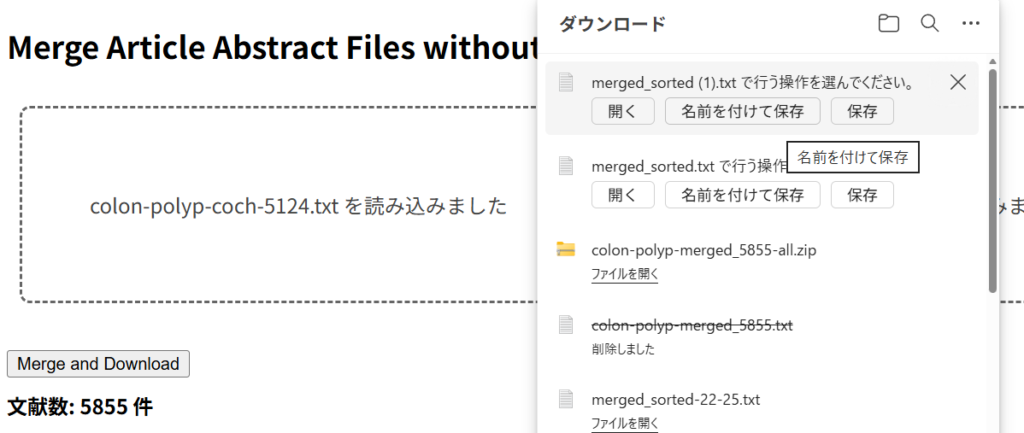
ドラッグアンドドロップのエリアが2つあるので、それぞれに上記のテキストファイルをドラッグアンドドロップする。下の図のような状態になるのでMerge and Downloadボタンをクリックする。
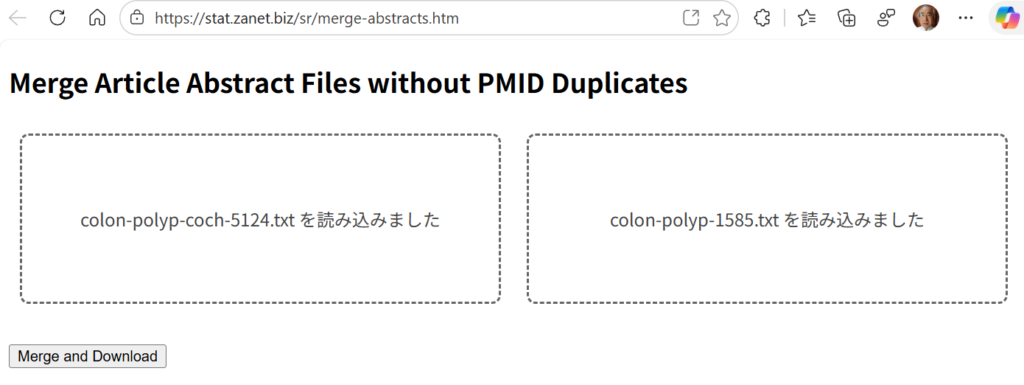
マージされた文献数が提示され、右上に名前を付けて保存のボタンが現れるので、クリックし、ファイル名を付けて保存する。このファイルには、2つのテキストファイルから重複を除いた文献が含まれている。
3つ以上のファイルをマージしたい場合は、保存したマージしたファイルを用いて、上記の作業を繰り返す。
7.文献数400ずつのファイルに分割する。
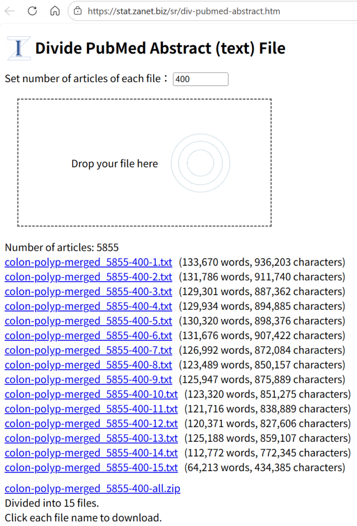
NLMでアップロードするファイルの大きさには制限があり、ある程度余裕も持たせて、400件ずつに分割することとする。分割には、ウェブツールであるDivide PubMed Abstract (text) Fileを用いる(著者作成)。
URL https://stat.zanet.biz/sr/div-pubmed-abstract.htm
元ファイルをドラッグアンドドロップすると、400件ずつのファイルに分割され、全部のファイルを含むZIPファイルも作成されるので、このZIPファイルをクリックして、名前を付けて保存する。
以上で、NLMにアップロードするファイルの準備ができた。以上の手順の内、時間を要するのは、文献検索であり、アブストラクトをダウンロードした後の操作は短時間で終了する。文献検索が重要なプロセスであり、網羅性を重視し、熟慮を重ね、トライアンドエラーで進める必要がある。
今回の例は、「大腸ポリープのポリペクトミー後のフォローアップはどれくらいの間隔で行うべきか?」がクエスチョンである。以下の2つの検索式を用いた。検索式1はPubMedのPublication typeを用い、検索式2はCochraneの感度最大化RCTフィルターを用いた。それぞれ、1585件、5124件の文献が引き出された。
検索式1:(“colonic polyps”[mh] OR “colorectal neoplasms”[mh] OR “colonic polyps”[tw]) AND (colonoscopy[mh] OR colonoscopy[tw] ) AND (follow-up OR aftercare[mh] OR “follow-up studies”[mh] OR surveillance[tiab]) AND (meta-analysis[pt] OR clinical trial[pt] OR comparative study[pt] OR multicenter study[pt] OR guideline[pt] OR systematic[sb]) AND humans[mh] AND (english[la] OR japanese[la]) AND hasabstract[tw]
検索式2:(“colonic polyps”[mh] OR “colorectal neoplasms”[mh] OR “colonic polyps”[tw]) AND (colonoscopy[mh] OR colonoscopy[tw] ) AND (english[la] OR japanese[la]) AND hasabstract[tw] AND (randomized controlled trial [pt] OR controlled clinical trial [pt] OR randomized [tiab] OR placebo [tiab] OR drug therapy [sh] OR randomly [tiab] OR trial [tiab] OR groups [tiab])
両者をマージした結果、5885件の文献が得られ、それを400件ずつの15のテキストファイルに分割した。
NLMの利用
ここからは、NLMのAIの利用プロセスに入る。
AIに何をさせたいのか?、何をアウトプットとして欲しいのかを十分考え、それを実現するプロンプトを作成する必要がある。
今回は、大腸ポリープ切除後のサーベイランスについて、フォローアップの間隔について調べようとしているので、以下のプロンプトを用いた。
あなたは、消化器病専門医、消化管内視鏡専門医です。ソースの情報に基づいて、大腸鏡でポリペクトミーを施行後フォローアップのための大腸鏡はどれくらいの間隔で施行すべきか、サーベイランスの方針についてまとめてください。ソースは3個の改行コードで区切られたブロックがひとつの文献です。それぞれのブロックの3行目が文献の書誌情報なので、引用した場合、その書誌情報の一覧を通し番号を付けて、最後に参考文献として付けてください。参考文献の書誌情報の最後はPMID: PMIDの番号となっていますが、PMIDの番号の文字列の後にスペースを入れ、続けて"https://pubmed.ncbi.nlm.nih.gov/" + "PMIDの番号"+"/"を書き入れてください。要点は、① ペルソナ、すなわち、誰が、あるいは誰のためにを指示すること、② 知りたいことを明確に述べる、③ 引用文献の書誌情報のリストの作成を指示したこと、である。
得られた回答は以下の通りである。
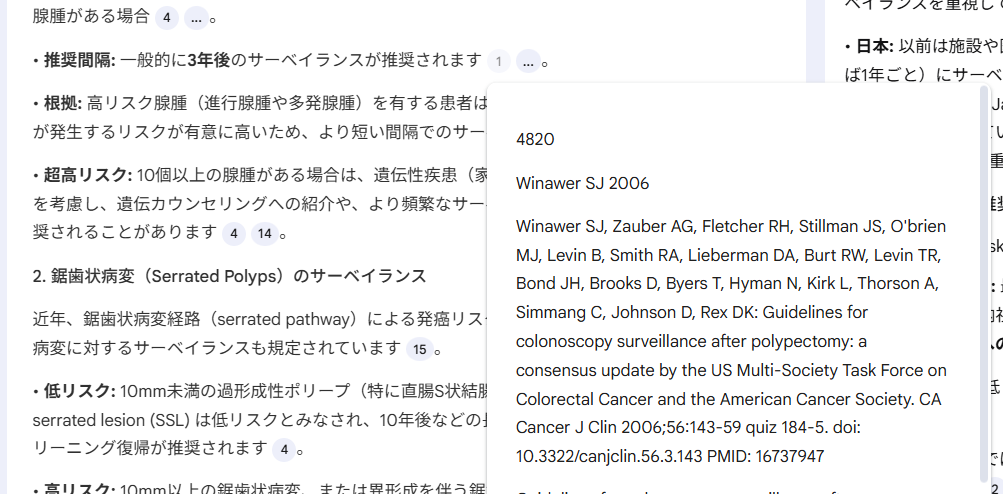
出力された回答には、参照したテキストの箇所を表示するための番号が振られた箇所があり、そこへマウスをホバリングするとその箇所がポップアップパネルに表示され、そこをクリックするとその箇所が左のパネルに表示される。下の図は前者の場合を示している。クリックした場合は、ソースの該当箇所が左のパネルに表示されるので、その前後もスクロールして確認することができる。また、この番号と巻末に付けられた文献リストの番号あるいは順番は同じではない。
回答が出力されると、下にメモに保存ボタンとコピーボタンが表示される。コピーボタンをクリックしてから、新規Googleドキュメントを開いて、そこに貼り付けて保存しておくことができる。以下に示すのは、Googleドキュメントの内容をコピーして貼り付けたものである。
また、メモに保存ボタンをクリックすると、右のStudioパネルにタイトルが表示されるようになるので、そこをクリックして、メモのタイトルを必要に応じて書き換えておく。保存したメモには、コピーボタンなどは無い。
チャットのパネルに示されたプロンプトに対する回答は、チャットのパネルの上にある、点が縦に3つ並んだボタンをクリックするとチャットの履歴を削除の操作をするまではそのまま残っており、以降のプロンプト実行時に参照される。
Googleドキュメントに貼り付けると、文献参照のURL部分の最後にカーソルをおいてスペースを追加すると、URLがアクティブになり、クリックすることで、小パネルが提示され、その中の青字の部分をクリックすると、PubMedの該当する文献のアブストラクトが開かれる。こうすることで、内容を確認することができる。
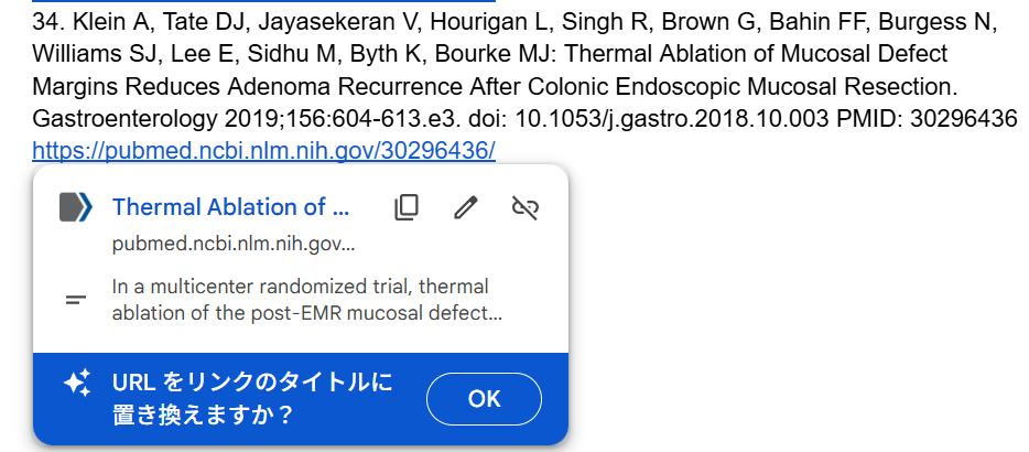
*この際に、URLをリンクのタイトルに置き換えますか?のOKボタンをクリックすると、URL部分がその論文のタイトルに置き換わり、そこをクリックするとPubMedの該当文献のアブストラクトが開かれるようになる。今回はその必要はないので、そのままにしておく。
以下に回答の全文を示す。
大腸ポリペクトミー後のサーベイランス
消化器病専門医および消化管内視鏡専門医の立場から、提供された文献に基づき、大腸内視鏡によるポリペクトミー後のサーベイランス(経過観察)方針についてまとめます。
サーベイランスの間隔は、初回内視鏡(ベースライン)で見つかったポリープの数、大きさ、組織型(腺腫か鋸歯状病変か)、および異形成の程度に基づく「リスク層別化」によって決定することが国際的なコンセンサスとなっています。
1. リスク層別化に基づくサーベイランス間隔
#低リスク群(Low Risk)
一般的に、少数の小さな腺腫のみが見つかった場合が該当します。
定義: 1~2個の管状腺腫で、大きさが10mm未満、かつ高度異形成(high-grade dysplasia)を伴わないもの。
推奨間隔: 多くのガイドラインでは、5年から10年後のサーベイランス、あるいはサーベイランスを行わず各国のスクリーニングプログラム(便潜血検査など)への復帰を推奨しています。
根拠: 低リスク腺腫切除後の進行性腫瘍(Advanced Neoplasia)の発生リスクは、ポリープがなかった群と比較して同等か、わずかに高い程度であり、頻繁な検査は不要とされています。米国(USMSTF)のガイドラインでは5~10年後、欧州(ESGE)や英国(BSG)のガイドラインでは、スクリーニングプログラムへの参加または10年後の大腸鏡が推奨されています。
微小ポリープの扱い: 5mm以下の微小腺腫(diminutive adenoma)と6-9mmの小腺腫(small adenoma)では、6-9mmの方が異時性進行病変のリスクが高いというデータがあり、微小腺腫のみの場合は間隔を延ばすことが検討されています。
#高リスク群(High Risk / Intermediate Risk)
進行した腺腫や多数の腺腫が見つかった場合が該当します。
定義:
進行腺腫(Advanced Adenoma):大きさが10mm以上、絨毛成分を含む、または高度異形成を伴うもの。
多発腺腫:ガイドラインにより定義が異なりますが、通常3個以上、あるいは5個以上の腺腫がある場合。
推奨間隔: 一般的に3年後のサーベイランスが推奨されます。
根拠: 高リスク腺腫(進行腺腫や多発腺腫)を有する患者は、将来的に進行性腫瘍や大腸癌が発生するリスクが有意に高いため、より短い間隔でのサーベイランスが必要です。
超高リスク: 10個以上の腺腫がある場合は、遺伝性疾患(家族性大腸腺腫症など)の可能性を考慮し、遺伝カウンセリングへの紹介や、より頻繁なサーベイランス(例:1年未満)が推奨されることがあります。
2. 鋸歯状病変(Serrated Polyps)のサーベイランス
近年、鋸歯状病変経路(serrated pathway)による発癌リスクが注目されており、これらの病変に対するサーベイランスも規定されています。
低リスク: 10mm未満の過形成性ポリープ(特に直腸S状結腸)や、異形成のないsessile serrated lesion (SSL) は低リスクとみなされ、10年後などの長期サーベイランスまたはスクリーニング復帰が推奨されます。
高リスク: 10mm以上の鋸歯状病変、または異形成を伴う鋸歯状病変(Traditional Serrated Adenomaを含む)は高リスクとみなされ、3年後のサーベイランスが推奨されます。
また、鋸歯状病変と通常の腺腫が併存する場合、進行腫瘍のリスクが増加するため、注意が必要です。
3. 分割切除(Piecemeal Resection)後のサーベイランス
20mmを超える大きな病変を内視鏡的粘膜切除術(EMR)などで分割切除した場合、局所再発のリスクが高くなります。
推奨方針: 切除から約6ヶ月後に最初のサーベイランス(SC1)を行い、遺残・再発がないか確認する必要があります。
長期経過: 最初のサーベイランスで再発がなければ、その後は1年後、3年後といった間隔で慎重に経過観察を行います。術後の熱凝固(スネアチップソフト凝固など)やクリップ閉鎖が再発率低下に寄与する可能性があります。
4. 大腸癌切除後のサーベイランス
大腸癌の根治切除後の患者も、異時性病変や局所再発のリスクがあるためサーベイランスが必要です。
推奨間隔: 術後1年後に大腸内視鏡を行い、異常がなければ次は3年後、その次は5年後と間隔を空けていくのが一般的です。
術前検査: 術前に閉塞などで全大腸の観察ができていない場合は、術後3~6ヶ月以内に残存結腸の検査を行うべきです。
5. その他の重要な考慮事項
腸管前処置(Bowel Preparation): 前処置が不良(Poor/Inadequate)で観察不十分な場合は、ガイドライン通りの間隔ではなく、1年以内など早期の再検査が必要です。
年齢と健康状態:
若年者(50歳未満): 若年で腺腫が見つかった場合でも、50歳以上と同様のリスク層別化に基づくサーベイランス間隔(低リスクなら5年、高リスクなら3年)が妥当であるという報告があります。
高齢者(75-80歳以上): 期待余命や併存疾患を考慮し、サーベイランスの中止を個別に検討すべきです。
検査の質(Quality of Colonoscopy): 腺腫発見率(ADR)が高い内視鏡医による検査や、適切な抜去時間(6分以上)の確保は、中間期癌のリスクを低減させるため、サーベイランス間隔の決定において前提となります。
まとめ
ポリペクトミー後のサーベイランスは、一律ではなく「リスクに応じた(Risk-stratified)」アプローチが必須です。
1. 低リスク(1-2個の<10mm管状腺腫): 5~10年後(またはスクリーニング復帰)。
2. 高リスク(≧3個、≧10mm、高度異形成/絨毛成分、または高リスク鋸歯状病変): 3年後。
3. 不完全切除・分割切除後: 6ヶ月後。
4. 大腸癌術後: 1年後。
これらの方針は、無駄な検査を減らしつつ、大腸癌の予防効果を最大化することを目的としています。
参考文献
1. Chen Y, Padilla Aponte J, Wang K, Du M, Lu Y, Polychronidis G, Song M: Comparative risk of high-risk neoplasia after polypectomy among individuals aged below 50 years versus 50 years and older. Gut 2025;75:72-80. doi: 10.1136/gutjnl-2025-335275 PMID: 40850745 https://pubmed.ncbi.nlm.nih.gov/40850745/
2. Uchiyama T, Takahashi H, Endo H, Kato S, Sakai E, Hosono K, Yoneda M, Inamori M, Hippo Y, Nakagama H, Nakajima A: Number of aberrant crypt foci in the rectum is a useful surrogate marker of colorectal adenoma recurrence. Dig Endosc 2012;24:353-7. doi: 10.1111/j.1443-1661.2012.01289.x PMID: 22925289 https://pubmed.ncbi.nlm.nih.gov/22925289/
3. Rex DK, Kahi CJ, Levin B, Smith RA, Bond JH, Brooks D, Burt RW, Byers T, Fletcher RH, Hyman N, Johnson D, Kirk L, Lieberman DA, Levin TR, O’Brien MJ, Simmang C, Thorson AG, Winawer SJ: Guidelines for colonoscopy surveillance after cancer resection: a consensus update by the American Cancer Society and US Multi-Society Task Force on Colorectal Cancer. CA Cancer J Clin 2006;56:160-7 quiz 185-6. doi: 10.3322/canjclin.56.3.160 PMID: 16737948 https://pubmed.ncbi.nlm.nih.gov/16737948/
4. Winawer SJ, Zauber AG, Fletcher RH, Stillman JS, O’brien MJ, Levin B, Smith RA, Lieberman DA, Burt RW, Levin TR, Bond JH, Brooks D, Byers T, Hyman N, Kirk L, Thorson A, Simmang C, Johnson D, Rex DK: Guidelines for colonoscopy surveillance after polypectomy: a consensus update by the US Multi-Society Task Force on Colorectal Cancer and the American Cancer Society. CA Cancer J Clin 2006;56:143-59 quiz 184-5. doi: 10.3322/canjclin.56.3.143 PMID: 16737947 https://pubmed.ncbi.nlm.nih.gov/16737947/
5. Rex DK, Kahi CJ, Levin B, Smith RA, Bond JH, Brooks D, Burt RW, Byers T, Fletcher RH, Hyman N, Johnson D, Kirk L, Lieberman DA, Levin TR, O’Brien MJ, Simmang C, Thorson AG, Winawer SJ, American Cancer Society, US Multi-Society Task Force on Colorectal Cancer: Guidelines for colonoscopy surveillance after cancer resection: a consensus update by the American Cancer Society and the US Multi-Society Task Force on Colorectal Cancer. Gastroenterology 2006;130:1865-71. doi: 10.1053/j.gastro.2006.03.013 PMID: 16697749 https://pubmed.ncbi.nlm.nih.gov/16697749/
6. Bobay MC, Lahr RE, Shultz J, Vemulapalli KC, Guardiola JJ, Rex DK: Safety of first surveillance colonoscopy at 12 months after piecemeal EMR of large nonpedunculated colorectal lesions. Gastrointest Endosc 2024;100:905-913. doi: 10.1016/j.gie.2024.05.008 PMID: 38750975 https://pubmed.ncbi.nlm.nih.gov/38750975/
7. Sasson AN, Sheehan G, Yu A, Gupta A, Ling K, Kochar B, Ananthakrishnan AN: Yield and Predictors of Surveillance Colonoscopies in Older Adults With Long-standing Ulcerative Colitis. Clin Gastroenterol Hepatol 2022;20:e1353-e1364. doi: 10.1016/j.cgh.2021.08.019 PMID: 34425278 https://pubmed.ncbi.nlm.nih.gov/34425278/
8. Waldmann E, Kammerlander A, Gessl I, Penz D, Majcher B, Hinterberger A, Trauner M, Ferlitsch M: New risk stratification after colorectal polypectomy reduces burden of surveillance without increasing mortality. United European Gastroenterol J 2021;9:947-954. doi: 10.1002/ueg2.12119 PMID: 34343405 https://pubmed.ncbi.nlm.nih.gov/34343405/
9. Symonds E, Anwar S, Young G, Meng R, Coats M, Simpson K, Bampton P, Fraser R, Cock C: Sessile Serrated Polyps with Synchronous Conventional Adenomas Increase Risk of Future Advanced Neoplasia. Dig Dis Sci 2019;64:1680-1685. doi: 10.1007/s10620-019-5454-8 PMID: 30627918 https://pubmed.ncbi.nlm.nih.gov/30627918/
10. Jung YS, Kim NH, Park JH, Park DI, Sohn CI: Appropriate Surveillance Interval after Colonoscopic Polypectomy in Patients Younger than 50 Years. J Korean Med Sci 2019;34:e101. doi: 10.3346/jkms.2019.34.e101 PMID: 30940997 https://pubmed.ncbi.nlm.nih.gov/30940997/
11. Rutter MD, East J, Rees CJ, Cripps N, Docherty J, Dolwani S, Kaye PV, Monahan KJ, Novelli MR, Plumb A, Saunders BP, Thomas-Gibson S, Tolan DJM, Whyte S, Bonnington S, Scope A, Wong R, Hibbert B, Marsh J, Moores B, Cross A, Sharp L: British Society of Gastroenterology/Association of Coloproctology of Great Britain and Ireland/Public Health England post-polypectomy and post-colorectal cancer resection surveillance guidelines. Gut 2020;69:201-223. doi: 10.1136/gutjnl-2019-319858 PMID: 31776230 https://pubmed.ncbi.nlm.nih.gov/31776230/
12. Parker J, Gupta S, Torkington J, Dolwani S: Comparison of recommendations for surveillance of advanced colorectal polyps: A systematic review of guidelines. J Gastroenterol Hepatol 2023;38:854-864. doi: 10.1111/jgh.16157 PMID: 36823764 https://pubmed.ncbi.nlm.nih.gov/36823764/
13. Lee JK, Jensen CD, Levin TR, Doubeni CA, Zauber AG, Chubak J, Kamineni AS, Schottinger JE, Ghai NR, Udaltsova N, Zhao WK, Fireman BH, Quesenberry CP, Orav EJ, Skinner CS, Halm EA, Corley DA: Long-term Risk of Colorectal Cancer and Related Death After Adenoma Removal in a Large, Community-based Population. Gastroenterology 2020;158:884-894.e5. doi: 10.1053/j.gastro.2019.09.039 PMID: 31589872 https://pubmed.ncbi.nlm.nih.gov/31589872/
14. Butterly LF, Nadel MR, Anderson JC, Robinson CM, Weiss JE, Lieberman D, Shapiro JA: Impact of Colonoscopy Bowel Preparation Quality on Follow-up Interval Recommendations for Average-risk Patients With Normal Screening Colonoscopies: Data From the New Hampshire Colonoscopy Registry. J Clin Gastroenterol 2020;54:356-364. doi: 10.1097/MCG.0000000000001115 PMID: 30106836 https://pubmed.ncbi.nlm.nih.gov/30106836/
15. East JE, Atkin WS, Bateman AC, Clark SK, Dolwani S, Ket SN, Leedham SJ, Phull PS, Rutter MD, Shepherd NA, Tomlinson I, Rees CJ: British Society of Gastroenterology position statement on serrated polyps in the colon and rectum. Gut 2017;66:1181-1196. doi: 10.1136/gutjnl-2017-314005 PMID: 28450390 https://pubmed.ncbi.nlm.nih.gov/28450390/
16. Nakajima T, Sakamoto T, Hori S, Yamada S, Ikematsu H, Harada K, Chiu HM, Kiriyama S, Michida T, Hotta K, Sakamoto N, Abe T, Chino A, Fukuzawa M, Kobayashi N, Fukase K, Matsuda T, Murakami Y, Ishikawa H, Saito Y: Optimal surveillance interval after piecemeal endoscopic mucosal resection for large colorectal neoplasia: a multicenter randomized controlled trial. Surg Endosc 2022;36:515-525. doi: 10.1007/s00464-021-08311-6 PMID: 33569725 https://pubmed.ncbi.nlm.nih.gov/33569725/
17. Jung YS, Kim TJ, Nam E, Park CH: Comparative systematic review and meta-analysis of 1- to 5-mm versus 6- to 9-mm adenomas on the risk of metachronous advanced colorectal neoplasia. Gastrointest Endosc 2020;92:692-701.e2. doi: 10.1016/j.gie.2020.04.042 PMID: 32334021 https://pubmed.ncbi.nlm.nih.gov/32334021/
18. Cross AJ, Robbins EC, Pack K, Stenson I, Kirby PL, Patel B, Rutter MD, Veitch AM, Saunders BP, Duffy SW, Wooldrage K: Long-term colorectal cancer incidence after adenoma removal and the effects of surveillance on incidence: a multicentre, retrospective, cohort study. Gut 2020;69:1645-1658. doi: 10.1136/gutjnl-2019-320036 PMID: 31953252 https://pubmed.ncbi.nlm.nih.gov/31953252/
19. Wieszczy P, Kaminski MF, Franczyk R, Loberg M, Kobiela J, Rupinska M, Kocot B, Rupinski M, Holme O, Wojciechowska U, Didkowska J, Ransohoff D, Bretthauer M, Kalager M, Regula J: Colorectal Cancer Incidence and Mortality After Removal of Adenomas During Screening Colonoscopies. Gastroenterology 2020;158:875-883.e5. doi: 10.1053/j.gastro.2019.09.011 PMID: 31563625 https://pubmed.ncbi.nlm.nih.gov/31563625/
20. Tate DJ, Desomer L, Klein A, Brown G, Hourigan LF, Lee EY, Moss A, Ormonde D, Raftopoulos S, Singh R, Williams SJ, Zanati S, Byth K, Bourke MJ: Adenoma recurrence after piecemeal colonic EMR is predictable: the Sydney EMR recurrence tool. Gastrointest Endosc 2017;85:647-656.e6. doi: 10.1016/j.gie.2016.11.027 PMID: 27908600 https://pubmed.ncbi.nlm.nih.gov/27908600/
21. Kahi CJ, Boland CR, Dominitz JA, Giardiello FM, Johnson DA, Kaltenbach T, Lieberman D, Levin TR, Robertson DJ, Rex DK, United States Multi-Society Task Force on Colorectal Cancer: Colonoscopy Surveillance After Colorectal Cancer Resection: Recommendations of the US Multi-Society Task Force on Colorectal Cancer. Gastroenterology 2016;150:758-768.e11. doi: 10.1053/j.gastro.2016.01.001 PMID: 26892199 https://pubmed.ncbi.nlm.nih.gov/26892199/
22. Kahi CJ, Boland CR, Dominitz JA, Giardiello FM, Johnson DA, Kaltenbach T, Lieberman D, Levin TR, Robertson DJ, Rex DK: Colonoscopy Surveillance after Colorectal Cancer Resection: Recommendations of the US Multi-Society Task Force on Colorectal Cancer. Am J Gastroenterol 2016;111:337-46 quiz 347. doi: 10.1038/ajg.2016.22 PMID: 26871541 https://pubmed.ncbi.nlm.nih.gov/26871541/
23. Jover R, Bretthauer M, Dekker E, Holme Ø, Kaminski MF, Løberg M, Zauber AG, Hernán MA, Lansdorp-Vogelaar I, Sunde A, McFadden E, Castells A, Regula J, Quintero E, Pellisé M, Senore C, Kalager M, Dinis-Ribeiro M, Emilsson L, Ransohoff DF, Hoff G, Adami HO: Rationale and design of the European Polyp Surveillance (EPoS) trials. Endoscopy 2016;48:571-8. doi: 10.1055/s-0042-104116 PMID: 27042931 https://pubmed.ncbi.nlm.nih.gov/27042931/
24. Clark BT, Rustagi T, Laine L: What level of bowel prep quality requires early repeat colonoscopy: systematic review and meta-analysis of the impact of preparation quality on adenoma detection rate. Am J Gastroenterol 2014;109:1714-23 quiz 1724. doi: 10.1038/ajg.2014.232 PMID: 25135006 https://pubmed.ncbi.nlm.nih.gov/25135006/
25. Hassan C, Quintero E, Dumonceau JM, Regula J, Brandão C, Chaussade S, Dekker E, Dinis-Ribeiro M, Ferlitsch M, Gimeno-García A, Hazewinkel Y, Jover R, Kalager M, Loberg M, Pox C, Rembacken B, Lieberman D, European Society of Gastrointestinal Endoscopy: Post-polypectomy colonoscopy surveillance: European Society of Gastrointestinal Endoscopy (ESGE) Guideline. Endoscopy 2013;45:842-51. doi: 10.1055/s-0033-1344548 PMID: 24030244 https://pubmed.ncbi.nlm.nih.gov/24030244/
26. Leddin D, Enns R, Hilsden R, Fallone CA, Rabeneck L, Sadowski DC, Singh H, Canadian Association of Gastroenterology: Colorectal cancer surveillance after index colonoscopy: guidance from the Canadian Association of Gastroenterology. Can J Gastroenterol 2013;27:224-8. doi: 10.1155/2013/232769 PMID: 23616961 https://pubmed.ncbi.nlm.nih.gov/23616961/
27. Winawer SJ, Zauber AG, O’Brien MJ, Ho MN, Gottlieb L, Sternberg SS, Waye JD, Bond J, Schapiro M, Stewart ET: Randomized comparison of surveillance intervals after colonoscopic removal of newly diagnosed adenomatous polyps. The National Polyp Study Workgroup. N Engl J Med 1993;328:901-6. doi: 10.1056/NEJM199304013281301 PMID: 8446136 https://pubmed.ncbi.nlm.nih.gov/8446136/
28. Winawer SJ, Zauber AG, Fletcher RH, Stillman JS, O’brien MJ, Levin B, Smith RA, Lieberman DA, Burt RW, Levin TR, Bond JH, Brooks D, Byers T, Hyman N, Kirk L, Thorson A, Simmang C, Johnson D, Rex DK: Guidelines for colonoscopy surveillance after polypectomy: a consensus update by the US Multi-Society Task Force on Colorectal Cancer and the American Cancer Society. CA Cancer J Clin 2006;56:143-59 quiz 184-5. doi: 10.3322/canjclin.56.3.143 PMID: 16737947 https://pubmed.ncbi.nlm.nih.gov/16737947/
29. Cross AJ, Robbins EC, Pack K, Stenson I, Rutter MD, Veitch AM, Saunders BP, Duffy SW, Wooldrage K: Colorectal cancer risk following polypectomy in a multicentre, retrospective, cohort study: an evaluation of the 2020 UK post-polypectomy surveillance guidelines. Gut 2021;70:2307-2320. doi: 10.1136/gutjnl-2020-323411 PMID: 33674342 https://pubmed.ncbi.nlm.nih.gov/33674342/
30. Kim NH, Jung YS, Park JH, Park DI, Sohn CI: Risk of developing metachronous advanced colorectal neoplasia after colonoscopic polypectomy in patients aged 30 to 39 and 40 to 49 years. Gastrointest Endosc 2018;88:715-723. doi: 10.1016/j.gie.2018.05.018 PMID: 29857003 https://pubmed.ncbi.nlm.nih.gov/29857003/
31. Pinsky PF, Schoen RE: Contribution of Surveillance Colonoscopy to Colorectal Cancer Prevention. Clin Gastroenterol Hepatol 2020;18:2937-2944.e1. doi: 10.1016/j.cgh.2020.01.037 PMID: 32017987 https://pubmed.ncbi.nlm.nih.gov/32017987/
32. Gupta S, Earles A, Bustamante R, Patterson OV, Gawron AJ, Kaltenbach TR, Yassin H, Lamm M, Shah SC, Saini SD, Fisher DA, Martinez ME, Messer K, Demb J, Liu L: Adenoma Detection Rate and Clinical Characteristics Influence Advanced Neoplasia Risk After Colorectal Polypectomy. Clin Gastroenterol Hepatol 2023;21:1924-1936.e9. doi: 10.1016/j.cgh.2022.10.003 PMID: 36270618 https://pubmed.ncbi.nlm.nih.gov/36270618/
33. Tate DJ, Desomer L, Hourigan LF, Moss A, Singh R, Bourke MJ: Two-stage endoscopic mucosal resection is a safe and effective salvage therapy after a failed single-session approach. Endoscopy 2017;49:888-898. doi: 10.1055/s-0043-110671 PMID: 28564715 https://pubmed.ncbi.nlm.nih.gov/28564715/ 34. Klein A, Tate DJ, Jayasekeran V, Hourigan L, Singh R, Brown G, Bahin FF, Burgess N, Williams SJ, Lee E, Sidhu M, Byth K, Bourke MJ: Thermal Ablation of Mucosal Defect Margins Reduces Adenoma Recurrence After Colonic Endoscopic Mucosal Resection. Gastroenterology 2019;156:604-613.e3. doi: 10.1053/j.gastro.2018.10.003 PMID: 30296436 https://pubmed.ncbi.nlm.nih.gov/30296436/
続いて、日本と欧米の方針の違いについて、以下のプロンプトで、調べることにした。
大腸ポリープ治療後のサーベイランス方針で日本と欧米の違いは?
ソースは3個の改行コードで区切られたブロックがひとつの文献です。それぞれのブロックの3行目が文献の書誌情報なので、引用した場合、その書誌情報の一覧を通し番号を付けて、最後に参考文献として付けてください。参考文献の書誌情報の最後はPMID: PMIDの番号となっていますが、PMIDの番号の文字列の後にスペースを入れ、続けて"https://pubmed.ncbi.nlm.nih.gov/" + "PMIDの番号"+"/"を書き入れてください。
得られた回答は以下の通りである。
大腸ポリペクトミー後のサーベイランス方針:日本と欧米の違い
大腸ポリープ治療後のサーベイランス方針で日本と欧米の違いは?
提供された文献情報に基づき、大腸ポリープ治療後のサーベイランス方針における日本と欧米の違いについてまとめます。
1. ガイドライン策定の背景と基本姿勢の違い
欧米と日本では、サーベイランスガイドラインの基盤となるエビデンスや基本理念に歴史的な違いがあります。
- 欧米(米国・欧州): 米国のNational Polyp Study (NPS) などのランダム化比較試験(RCT)の結果に基づき、早期からリスク層別化によるサーベイランス間隔の延長(3年、5年、10年など)を推奨してきました。限られた内視鏡資源や医療コストを考慮し、リスクに応じた効率的なサーベイランスを重視しています。
- 日本: 以前は施設や医師ごとに方針が委ねられており、欧米のガイドラインよりも頻繁(例えば1年ごと)にサーベイランスを行う傾向がありました。しかし、近年では日本で行われた大規模RCTである**Japan Polyp Study (JPS)**のエビデンスが確立され、これに基づいたガイドラインが策定されています。日本のガイドラインは「サーベイランス中の大腸癌死ゼロ」「腸管温存」「患者のQOL重視」を基本原則としています。
2. リスク層別化と推奨間隔の比較
低リスク群 (Low Risk)
- 欧州 (ESGE/BSG): 最新のガイドラインでは、低リスク腺腫(1-2個の10mm未満の管状腺腫など)の切除後は、内視鏡によるサーベイランスを行わず、便潜血検査(FIT)を用いたスクリーニングプログラムへの復帰を推奨するなど、サーベイランスの抑制に積極的です。
- 米国 (USMSTF): 低リスク群に対しては、7~10年後(以前は5-10年)のサーベイランスを推奨しています。
- 日本: 過去の調査では、低リスク腺腫であっても多くの医師が米国よりも短い間隔での検査を推奨していました。しかし、JPSの結果により、高リスク群であっても適切な切除(クリーンコロン化)が行われれば3年後のサーベイランスで大腸癌リスクを抑制できることが示されており、無駄な検査を減らす方向性が示唆されています。
高リスク群 (High Risk)
- 共通点: 進行腺腫(10mm以上、絨毛成分、高度異形成)や多発腺腫(3個以上など)を持つ高リスク群に対しては、日米欧ともに3年後のサーベイランスを推奨する点で概ね一致しています。
- 定義の微細な違い:
- 英国 (BSG/ACPGBI): 2020年のガイドライン等では、腺腫の個数(5個以上など)や大きさだけでなく、これらの組み合わせでリスクを定義し、高リスク患者には3年後の検査を推奨する一方、低リスク患者にはサーベイランス不要(スクリーニングへ移行)とするなど、よりメリハリのある管理を提案しています。
- 米国: 10mm以上の鋸歯状病変(Serrated polyps)や異形成を伴うものも高リスクとして3年後のフォローを推奨しています。
3. 鋸歯状病変 (Serrated Lesions) への対応
鋸歯状病変(SSLなど)は「serrated pathway」による発癌リスクがあるため、欧米のガイドラインでは具体的なサーベイランス間隔が規定されています。
- 米国 (USMSTF): 10mm未満のSSLが1-2個なら5-10年後、3-4個なら3-5年後と細かく規定しています。
- 欧州 (ESGE): 以前は詳細な規定が少なかったものの、近年の改訂で鋸歯状病変もリスク分類に取り入れられています。
- 日本: 表面型腫瘍(non-polypoid colorectal neoplasms: NP-CRNs)の診断・治療に長けており、JPSの結果でも、発見された進行病変の半数以上がNP-CRN(平坦・陥凹型、側方発育型など)であったことが報告されています。日本はこの分野の内視鏡診断・治療技術が進んでおり、これらの病変を含めた「クリーンコロン」の達成を前提としたサーベイランスが重視されます。
4. まとめ
- 欧米: 公衆衛生的な観点から、低リスク群のサーベイランスを省略・延長し(FITへの移行など)、リソースを高リスク群に集中させる傾向が強いです。
- 日本: 従来は慎重な(頻繁な)フォローアップが行われてきましたが、Japan Polyp Studyのエビデンスにより、初回治療でしっかり病変を取りきること(クリーンコロン)を前提に、サーベイランス間隔を欧米同様に延長(3年後など)する方針が科学的に裏付けられました。
参考文献
Hotta K, Matsuda T, Sano Y, Fujii T, Saito Y: Surveillance after Endoscopic Resection for Colorectal Tumors: A Comprehensive Review. Digestion 2025;106:131-137. doi: 10.1159/000542665 PMID: 39571558 https://pubmed.ncbi.nlm.nih.gov/39571558/
Tanaka S, Obata D, Chinzei R, Yoshida S, Sanuki T, Morita Y, Yoshida M, Fujita T, Toyonaga T, Kutsumi H, Inokuchi H, Azuma T: Surveillance after colorectal polypectomy; comparison between Japan and U.S. Kobe J Med Sci 2011;56:E204-13. PMID: 21937868 https://pubmed.ncbi.nlm.nih.gov/21937868/
Sano Y, Hotta K, Matsuda T, Murakami Y, Fujii T, Kudo SE, Oda Y, Ishikawa H, Saito Y, Kobayashi N, Sekiguchi M, Ikematsu H, Katagiri A, Konishi K, Takeuchi Y, Iishi H, Igarashi M, Kobayashi K, Sada M, Osera S, Shinohara T, Yamaguchi Y, Hasuda K, Morishima T, Miyashiro I, Shimoda T, Taniguchi H, Fujimori T, Ajioka Y, Yoshida S, Japan Polyp Study Workgroup: Endoscopic Removal of Premalignant Lesions Reduces Long-Term Colorectal Cancer Risk: Results From the Japan Polyp Study. Clin Gastroenterol Hepatol 2024;22:542-551.e3. doi: 10.1016/j.cgh.2023.07.021 PMID: 37544420 https://pubmed.ncbi.nlm.nih.gov/37544420/
Abu-Freha N, Katz LH, Kariv R, Vainer E, Laish I, Gluck N, Half EE, Levi Z: Post-polypectomy surveillance colonoscopy: Comparison of the updated guidelines. United European Gastroenterol J 2021;9:681-687. doi: 10.1002/ueg2.12106 PMID: 34077635 https://pubmed.ncbi.nlm.nih.gov/34077635/
Cross AJ, Robbins EC, Pack K, Stenson I, Patel B, Rutter MD, Veitch AM, Saunders BP, Duffy SW, Wooldrage K: Colorectal cancer risk following polypectomy in a multicentre, retrospective, cohort study: an evaluation of the 2020 UK post-polypectomy surveillance guidelines. Gut 2021;70:2307-2320. doi: 10.1136/gutjnl-2020-323411 PMID: 33674342 https://pubmed.ncbi.nlm.nih.gov/33674342/Park SK, Yang HJ, Jung YS, Park JH, Sohn CI, Park DI: Risk of advanced colorectal neoplasm by the proposed combined United States and United Kingdom risk stratification guidelines. Gastrointest Endosc 2018;87:800-808. doi: 10.1016/j.gie.2017.09.023 PMID: 28986265 https://pubmed.ncbi.nlm.nih.gov/28986265/
今回は、参照文献に通し番号が付けられていなかった。この例のように、AIがすべて指示通りの作業をしてくれるとは限らない。また、同じプロンプトを別の機会に実行すると、表現に少し違いがあったりする。しかし、内容はほぼ同じであった。
結果の精度を調べる
今回の例では、日本消化器病学会から2020年に大腸ポリープ診療ガイドラインが発行されており、PDFファイルが公開されているので、それを参照してみると、CO7-1 大腸腺腫の内視鏡切除後のサ-ベイランスはどうすべきか?が今回のテーマに該当する。その内容は以下の通りである。
CQ7-1 大腸腺腫の内視鏡切除後のサーベイランスはどうすべきか?
日本消化器病学会:大腸ポリープ診療ガイドライン。2020年版
推奨
大腸腺腫性ポリ-プに対する内視鏡切除後のサ-ベイランス内視鏡検査は,3年以内に行うことを提案する.
【推奨の強さ:弱(合意率100%),エビデンスレベル:B】
解説
米国NationaPolypStudyより,大腸腺腫性ポリ-プを内視鏡的にすべて切除することで,その後のサ-ベイランス内視鏡検査は3年後と推奨された。また,初回の全大腸内視鏡検査所見に基づき,その後約5年間でのadvanced neoplasia(径10mm以上の腺腫,villous tumor,high grade dysplasiaあるいは痛)の累積発生率が報告され,初回の全大腸内視鏡検査所見の重要性が示さきれた(表1)。
European guideline 3および米国guideline改訂版に従えば,全大腸内視鏡検査における腺腫性ポリ-プの個数と最大径,病理組織診断(villous成分とhigh grade dysplasiaの有無)により,それぞれ推奨すべき全大腸内視鏡検査間隔が決められている.基本的に径10mm以下の腺腫性ポリ-プ(low grade dysplasia)を3個以上,あるいはhigh grade dysplasiaやvillous成分を有するポリ-プを内視鏡的に切除した場合には,一律3年後のサ-ベイランス全大腸内視鏡検査が推奨されている.さらに,径10mm以下のlow grade dysplasiaが2個までの場合には,European guidelineでは10年後のroutine screening(通常の便潜血などのスクリ-ニング)を,米国guidelineでは5一10年後の全大腸内視鏡検査が推奨されている.その他,腺腫性ポリ-プが多数(10個以上)認められる場合や鋸歯状病変が認められた場合など,初回の全大腸内視鏡検査所見によって詳細なリスク層別化がなされ,それぞれに推奨される全大腸内視鏡検査間隔が定められている.
日本では,いまだ径5mm以下の腺腫性ポリ-プの取り扱いが一定でないため,海外のガイドラインをそのまま適応してよいかどうかは明らかではない.つまり,発見した腺腫性ポリ-プをすべて切除することが強く推奨されている欧米と,担癌率の極めて低い径5mm以下のポリ-プについては,切除せずに経過観察してもよいとする本邦の立場が異なるため,サ-ベイランス全大腸内視鏡検査間隔については一定の見解が得られていない。そこで,本CQに対しては,Japan Polyp Study Workgroupの遡及的検討結果(1回の完全なポリ-プ切除では,検査間隔を一律3年後に設定することの安全性が十分担保できない”という結論)に基づき,本推奨とした。今後,Japan Polyp Studyの長期追跡デ-タが待たれる.
この中に、Japan Polyp Studyの結果が待たれるという記述があり、上記の日本と欧米の方針の違いについての回答の参照文献にあるSano Y 2024がそれに相当すると思われる。そこで、この文献へのリンクを開き、PubMedのアブストラクトのページから出版社へのリンクを開くと全文が公開されていた。
さて、今度はGemniを使って、以下のプロンプトを実行してみる。
日本消化器病学会の大腸ポリープ診療ガイドラインは2020年に発刊されています。その後、Japan Polyp Studyの結果が2024年に発表され(Clin Gastroenterol Hepatol 2024;22:542-551.)、CO7-1 大腸腺腫の内視鏡切除後のサ-ベイランスはどうすべきか?について変更がなされていますか?すると、この診療ガイドラインの改訂版はまだ発刊されていないこと、Japan Polyp Studyの結果を踏まえた方針の変更の可能性について言及されていた。
JPS後の議論
ご指摘の通り、2020年のガイドライン発刊後、日本の大規模臨床試験である Japan Polyp Study (JPS) の解析結果が発表されたことで、大腸ポリープ切除後のフォローアップ(サーベイランス)の考え方に重要な知見が加わりました。
結論から申し上げますと、現時点で学会公式の「ガイドライン」そのものが改訂・出版されたわけではありませんが、JPSの結果を受けて、**「クリーンコロン(すべてのポリープを摘出した状態)が得られれば、低リスク群ではサーベイランスの間隔を延長できる可能性がある」**という方向で議論が進んでいます。
以下に、JPSの結果を踏まえた変更点やポイントを整理しました。
1. Japan Polyp Study (JPS) 2024年報告の要旨
JPSは、内視鏡除外後のサーベイランス間隔を「1年後+3年後(計2回)」群と、「3年後のみ(1回)」群で比較したランダム化比較試験です。
- 主な結果: 3年後に発見される進行大腸癌や高度腺腫の発生率は、両群間で有意差がありませんでした。
- 結論: 適切な初回内視鏡(高品質な検査)でポリープを完全に切除できていれば、翌年の検査をスキップして3年後としても安全性は損なわれないことが示唆されました。
2. ガイドライン(2020年版)とJPS後の考え方の比較
現行のガイドライン(CQ7-1)の推奨と、JPSの結果を受けた現在の専門医のコンセンサスを比較します。
| 項目 | 2020年ガイドライン (CQ7-1) | JPS発表後(現在の動向) |
| 基本的な推奨 | 摘除後1〜3年以内のサーベイランスを推奨 | クリーンコロン達成後は間隔を延ばす傾向 |
| 低リスク群 (1-2個, 小腺腫) | 3年後の検査を考慮してもよい | **3年(あるいはそれ以上)**の間隔が妥当 |
| 高リスク群 (3個以上, 大腺腫) | 1年後の検査を推奨 | 依然として1年〜2年後の慎重な観察が主流 |
| 検査の質 | 言及はあるが具体性に欠ける | **「高品質な初回内視鏡」**の重要性がより強調される |
3. 実臨床における具体的な変更点
JPSの結果(2024年)を受けて、特に以下の点が臨床現場で重視されるようになっています。
- 「1年後」の全例実施の見直し: 2020年版では「1〜3年」と幅がありましたが、小さなポリープが1、2個だった患者さんに対し、一律に「念のため来年も」と勧めるケースが減り、3年後への延長を提示しやすくなりました。
- 「質の高い内視鏡」の前提: JPSの結果は、熟練医が盲腸まで到達し、十分な観察時間をかけ、全ての腫瘍性病変を摘出したことが前提です。そのため、便の残りが多かった場合や、観察が不十分だった場合は、従来通り1年以内の再検が求められます。
まとめ
公式なガイドラインの「書籍」としての改訂はまだですが、JPS 2024の結果は**「低リスク症例におけるサーベイランス間隔の延長」**を強く後押しするエビデンスとなりました。これにより、患者さんの身体的・経済的負担を軽減し、医療資源をより高リスクな患者へ集中させる効率的な医療へのシフトが進んでいます。
もし、特定の症例(ポリープの数や大きさ、組織型など)について、JPSの基準に照らし合わせた具体的な判断基準をお知りになりたい場合は、続けてお知らせください。
ここまでの検討で、NLMを使用することで実用的な情報を高精度で得られることが分かった。今後、さまざまなテーマであるいはクエスチョンでNLMの性能を評価する必要があるだろう。