連続変数アウトカムで平均値差Mean Difference, MDまたは標準化平均値差Standardized Mean Difference (SMD)の統合値と95%確信区間Credible Intervalを、Stanを用いてベイジアンメタアナリシスで求め、Forest plotを作成するコードです。
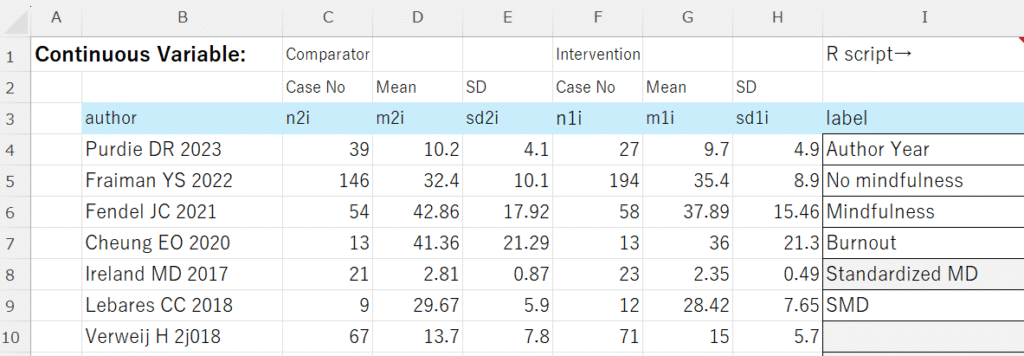
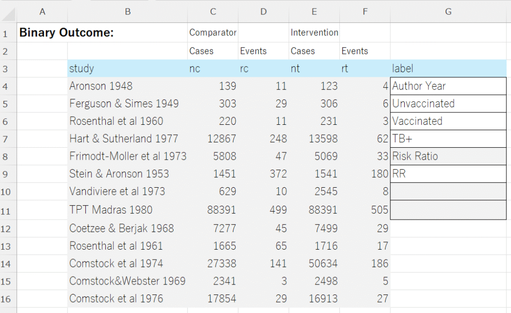
データはExcelで図のように準備します。labelは研究名のラベル、対照、介入のラベル、アウトカム、効果指標のタイプ、その略称です。セルI9がMDの場合は、平均値差、SMDの場合は標準化平均値差を計算します。この例ではSMDを計算します。
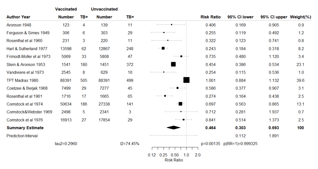
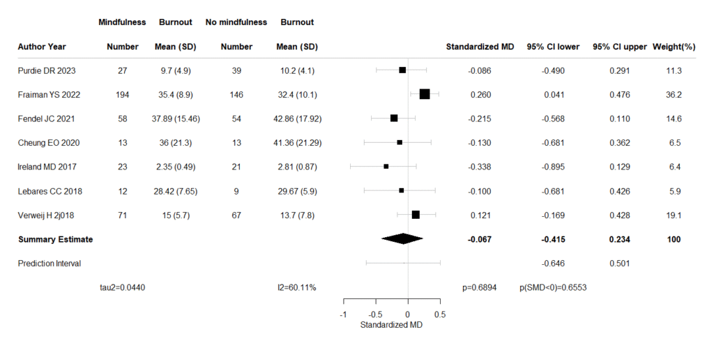
Rを起動しておき、エディターにコピーした下記コードを貼り付けて、最初の5つのライブラリの読み込みを実行しておきます。Excelに戻って、セルB3からI10までの範囲を選択して、コピー操作(Ctrl+C)を行って、Rに戻り、exdato = read.delim(“clipboard”,sep=”\t”,header=TRUE)のスクリプトを実行します。続いて、それ以下のスクリプトを全部実行させると、Forest plotが出力されます。効果指標の点推定値と95%確信区間、および予測区間を提示します。
Markov Chain Monte Carlo (MCMC)シミュレーションを行うので、少し時間がかかります。chains = 4, warmup = 10000, iter = 20000に設定しているので、計40000個がサンプリングされます。
Forest plotが出力された時点で、各研究の効果推定値、95%確信区間、統合値と95%確信区間、予測区間の値をクリップボードにコピーしていますので、Excel評価シートなどに貼り付けることができます。
平均値差MD、標準化平均値差SMDのメタアナリシス用コード
#####MD and SMD Bayesian meta-analysis with Stan, rstan######
# R code for data preparation
library(rstan)
library(bayesplot)
library(dplyr)
library(HDInterval)
library(forestplot)
library(metafor)
# Get data via clipboard from Excel sheet.
exdato = read.delim("clipboard",sep="\t",header=TRUE)
labem = exdato[,"label"]
em = labem[6]
labe_study = labem[1]
labe_cont = labem[2]
labe_int = labem[3]
labe_outc = labem[4]
labe_em = labem[5]
exdat=na.omit(exdato)
# Number of studies
K <- nrow(exdat)
# Calculate individual study effect sizes (MD and SMD) and their variances
# For Mean Difference (MD)
exdat$yi_md <- exdat$m1i - exdat$m2i
exdat$vi_md <- (exdat$sd1i^2 / exdat$n1i) + (exdat$sd2i^2 / exdat$n2i)
exdat$sei_md <- sqrt(exdat$vi_md)
# For Standardized Mean Difference (SMD) - using Hedges' g approximation
# Calculate pooled standard deviation
exdat$sd_pooled <- with(exdat, sqrt(((n1i - 1) * sd1i^2 + (n2i - 1) * sd2i^2) / (n1i + n2i - 2)))
exdat$yi_smd <- (exdat$m1i - exdat$m2i) / exdat$sd_pooled
# Calculate variance for SMD (Hedges' g)
exdat$vi_smd <- with(exdat, ((n1i + n2i) / (n1i * n2i)) + (yi_smd^2 / (2 * (n1i + n2i))))
exdat$sei_smd <- sqrt(exdat$vi_smd)
if(em=="MD"){
# Stan data for MD
stan_data_md <- list(
K = K,
yi = exdat$yi_md,
sei = exdat$sei_md
)
}
if(em=="SMD"){
# Stan data for SMD
stan_data_smd <- list(
K = K,
yi = exdat$yi_smd,
sei = exdat$sei_smd
)
}
######
if(em=="MD"){
## Stan code for Mean Difference (MD) random-effects model
stan_md_code <- "
data {
int<lower=0> K; // number of studies
array[K] real yi; // observed effect sizes
array[K] real<lower=0> sei; // standard errors of effect sizes
}
parameters {
real mu; // overall mean effect
real<lower=0> tau; // between-study standard deviation
array[K] real delta; // true effect size for each study
}
transformed parameters {
real<lower=0> tau_squared; // between-study variance
real<lower=0,upper=1> I_squared; // I-squared statistic
tau_squared = square(tau);
// Calculate I-squared
// Average sampling variance (approximation)
real var_sampling_avg = mean(square(sei));
I_squared = tau_squared / (tau_squared + var_sampling_avg);
}
model {
// Priors
mu ~ normal(0, 10); // weakly informative prior for overall mean
tau ~ normal(0, 1); // weakly informative prior for tau (sd of random effects)
// Likelihood
delta ~ normal(mu, tau); // true effect sizes drawn from a normal distribution
yi ~ normal(delta, sei); // observed effect sizes are normally distributed around true effect sizes
}
generated quantities {
real prediction_interval_lower;
real prediction_interval_upper;
real new_delta; // New true effect size from the meta-analytic distribution
// Prediction interval for a new study's true effect size
new_delta = normal_rng(mu, tau);
// To get the interval, we sample many 'new_delta' and take quantiles later
// For simplicity, we can also directly calculate it if mu and tau are well-behaved.
// However, for a true Bayesian prediction interval, it's best to sample.
// Here, for outputting directly from Stan, we can use quantiles of posterior samples of mu and tau
// and combine them, or draw samples as below.
// For a direct 95% interval, we can compute it from mu and tau:
prediction_interval_lower = mu - 1.96 * tau;
prediction_interval_upper = mu + 1.96 * tau;
}
"
}
#####
if(em == "SMD"){
## Stan code for Standardized Mean Difference (SMD) random-effects model
stan_smd_code <- "
data {
int<lower=0> K; // number of studies
array[K] real yi; // observed effect sizes (SMD)
array[K] real<lower=0> sei; // standard errors of effect sizes
}
parameters {
real mu; // overall mean effect (SMD)
real<lower=0> tau; // between-study standard deviation
array[K] real delta; // true effect size for each study
}
transformed parameters {
real<lower=0> tau_squared; // between-study variance
real<lower=0,upper=1> I_squared; // I-squared statistic
tau_squared = square(tau);
// Calculate I-squared
// Average sampling variance (approximation)
real var_sampling_avg = mean(square(sei));
I_squared = tau_squared / (tau_squared + var_sampling_avg);
}
model {
// Priors
mu ~ normal(0, 1); // weakly informative prior for overall mean (SMD is typically smaller scale)
tau ~ normal(0, 0.5); // weakly informative prior for tau (sd of random effects, typically smaller for SMD)
// Likelihood
delta ~ normal(mu, tau); // true effect sizes drawn from a normal distribution
yi ~ normal(delta, sei); // observed effect sizes are normally distributed around true effect sizes
}
generated quantities {
real prediction_interval_lower;
real prediction_interval_upper;
real new_delta; // New true effect size from the meta-analytic distribution
// Prediction interval for a new study's true effect size
new_delta = normal_rng(mu, tau);
prediction_interval_lower = mu - 1.96 * tau;
prediction_interval_upper = mu + 1.96 * tau;
}
"
}
#####
# R code to run Stan models and extract results
if(em=="MD"){
# Compile the MD Stan model
stan_md_model <- stan_model(model_code = stan_md_code)
# Run the MD model
fit_md <- sampling(stan_md_model,
data = stan_data_md,
chains = 4, # number of MCMC chains
iter = 20000, # number of iterations per chain
warmup = 10000, # warmup iterations
thin = 1, # thinning rate
seed = 1234, # for reproducibility
control = list(adapt_delta = 0.95, max_treedepth = 15)) # improve sampling
print(fit_md, pars = c("mu", "tau", "tau_squared", "I_squared", "prediction_interval_lower", "prediction_interval_upper"),
probs = c(0.025, 0.5, 0.975))
# Plotting (optional)
# dev.new();mcmc_dens(fit_md, pars = c("mu", "tau", "tau_squared", "I_squared"))
# dev.new();mcmc_trace(fit_md, pars = c("mu", "tau"))
}
###
if(em=="SMD"){
# Compile the SMD Stan model
stan_smd_model <- stan_model(model_code = stan_smd_code)
# Run the SMD model
fit_smd <- sampling(stan_smd_model,
data = stan_data_smd,
chains = 4,
iter = 20000,
warmup = 10000,
thin = 1,
seed = 1234,
control = list(adapt_delta = 0.95, max_treedepth = 15))
print(fit_smd, pars = c("mu", "tau", "tau_squared", "I_squared", "prediction_interval_lower", "prediction_interval_upper"),
probs = c(0.025, 0.5, 0.975))
# Plotting (optional)
# dev.new();mcmc_dens(fit_smd, pars = c("mu", "tau", "tau_squared", "I_squared"))
# dev.new();mcmc_trace(fit_smd, pars = c("mu", "tau"))
}
#####
if(em=="MD"){
#Posterior samples of MD
posterior_samples=extract(fit_md)
#md meand difference
mu_md=mean(posterior_samples$mu)
mu_md_ci=quantile(posterior_samples$mu,probs=c(0.025,0.975))
mu_md_lw=mu_md_ci[1]
mu_md_up=mu_md_ci[2]
p_val_md = round(2*min(mean(posterior_samples$mu >0), mean(posterior_samples$mu <0)), 6) #Bayesian p-value for summary MD
if(mu_md>0){
prob_direct_md = round(mean(posterior_samples$mu > 0),6)
label = "p(MD>0)="
}else{
prob_direct_md = round(mean(posterior_samples$mu < 0),6)
label = "p(MD<0)="
}
#md tau-squared
#if normal distribution.
#mu_md_tau_squared=mean(posterior_samples$tau_squared)
#mu_md_tau_squared_ci=quantile(posterior_samples$tau_squared,probs=c(0.025,0.975))
#mu_md_tau_squared_lw=mu_md_tau_squared_ci[1]
#mu_md_tau_squared_up=mu_md_tau_squared_ci[2]
#if skewed distributions.
dens=density(posterior_samples$tau_squared)
mu_md_tau_squared=dens$x[which.max(dens$y)] #mode
mu_md_tau_squared_lw=hdi(posterior_samples$tau_squared)[1] #High Density Interval (HDI) lower
mu_md_tau_squared_up=hdi(posterior_samples$tau_squared)[2] #High Density Interval (HDI) upper
#md I-squared
#if normal distribution.
#mu_md_I_squared=mean(posterior_samples$I_squared)
#mu_md_I_squared_ci=quantile(posterior_samples$I_squared,probs=c(0.025,0.975))
#mu_md_I_squared_lw=mu_md_I_squared_ci[1]
#mu_md_I_squared_up=mu_md_I_squared_ci[2]
#if skewed distributions.
dens=density(posterior_samples$I_squared)
mu_md_I_squared=dens$x[which.max(dens$y)] #mode
mu_md_I_squared_lw=hdi(posterior_samples$I_squared)[1] #High Density Interval (HDI) lower
mu_md_I_squared_up=hdi(posterior_samples$I_squared)[2] #High Density Interval (HDI) upper
#md Prediction Interval
mu_new_md=mean(posterior_samples$new_delta)
mu_new_md_ci=quantile(posterior_samples$new_delta,probs=c(0.025,0.975))
mu_md_pi_lw=median(posterior_samples$prediction_interval_lower)
mu_md_pi_up=median(posterior_samples$prediction_interval_upper)
}
####
if(em=="SMD"){
#Posterior samples of SMD
posterior_samples=extract(fit_smd)
#smd meand difference
mu_smd=mean(posterior_samples$mu)
mu_smd_ci=quantile(posterior_samples$mu,probs=c(0.025,0.975))
mu_smd_lw=mu_smd_ci[1]
mu_smd_up=mu_smd_ci[2]
p_val_smd = round(2*min(mean(posterior_samples$mu >0), mean(posterior_samples$mu <0)), 6) #Bayesian p-value for summary MD
if(mu_smd>0){
prob_direct_smd = round(mean(posterior_samples$mu > 0),6)
label = "p(SMD>0)="
}else{
prob_direct_smd = round(mean(posterior_samples$mu < 0),6)
label = "p(SMD<0)="
}
#smd tau-squared
#if normal distribution.
#mu_smd_tau_squared=mean(posterior_samples$tau_squared) #mean
#mu_smd_tau_squared_ci=quantile(posterior_samples$tau_squared,probs=c(0.025,0.975))
#mu_smd_tau_squared_lw=mu_smd_tau_squared_ci[1]
#mu_smd_tau_squared_up=mu_smd_tau_squared_ci[2]
#if skewed distributions.
dens=density(posterior_samples$tau_squared)
mu_smd_tau_squared=dens$x[which.max(dens$y)] #mode
mu_smd_tau_squared_lw=hdi(posterior_samples$tau_squared)[1] #High Density Interval (HDI) lower
mu_smd_tau_squared_up=hdi(posterior_samples$tau_squared)[2] #High Density Interval (HDI) upper
#smd I-squared
#if normal distribution.
#mu_smd_I_squared=mean(posterior_samples$I_squared)
#mu_smd_I_squared_ci=quantile(posterior_samples$I_squared,probs=c(0.025,0.975))
#mu_smd_I_squared_lw=mu_smd_I_squared_ci[1]
#mu_smd_I_squared_up=mu_smd_I_squared_ci[2]
#if skewed distributions.
dens=density(posterior_samples$I_squared)
mu_smd_I_squared=dens$x[which.max(dens$y)] #mode
mu_smd_I_squared_lw=hdi(posterior_samples$I_squared)[1] #High Density Interval (HDI) lower
mu_smd_I_squared_up=hdi(posterior_samples$I_squared)[2] #High Density Interval (HDI) upper
#smd Prediction Interval
mu_new_smd=mean(posterior_samples$new_delta)
mu_new_smd_ci=quantile(posterior_samples$new_delta,probs=c(0.025,0.975))
mu_smd_pi_lw=median(posterior_samples$prediction_interval_lower)
mu_smd_pi_up=median(posterior_samples$prediction_interval_upper)
}
#####
if(em=="MD"){
#各研究のmdと95%CI
md=rep(0,K)
md_lw=md
md_up=md
for(i in 1:K){
md[i]=mean(posterior_samples$delta[,i])
md_lw[i]=quantile(posterior_samples$delta[,i],probs=0.025)
md_up[i]=quantile(posterior_samples$delta[,i],probs=0.975)
}
}
if(em=="SMD"){
#各研究のsmdと95%CI
smd=rep(0,K)
smd_lw=smd
smd_up=smd
for(i in 1:K){
smd[i]=mean(posterior_samples$delta[,i])
smd_lw[i]=quantile(posterior_samples$delta[,i],probs=0.025)
smd_up[i]=quantile(posterior_samples$delta[,i],probs=0.975)
}
}
#########
#Forest Plot
if(em=="MD"){
#MD
# 重みを格納するベクトルを初期化
weights <- numeric(K)
weight_percentages <- numeric(K)
for (i in 1:K) {
# i番目の研究のmdのサンプリング値を取得
md_i_samples <- posterior_samples$delta[, i]
# そのサンプリングされた値の分散を計算
# これを「実効的な逆分散」と考える
variance_of_md_i <- var(md_i_samples)
# 重みは分散の逆数
weights[i] <- 1 / variance_of_md_i
}
# 全重みの合計
total_weight <- sum(weights)
# 各研究の重みのパーセンテージ
weight_percentages <- (weights / total_weight) * 100
# 結果の表示
results_weights_posterior_var <- data.frame(
Study = 1:K,
Effective_Weight = weights,
Effective_Weight_Percentage = weight_percentages
)
print(results_weights_posterior_var)
k=K
wpc = format(round(weight_percentages,digits=1), nsmall=1)
wp = weight_percentages/100
#Forest plot box sizes on weihts
wbox=c(NA,NA,(k/4)*sqrt(wp)/sum(sqrt(wp)),0.5,0,NA)
#setting fs for cex
fs=1
if(k>20){fs=round((1-0.02*(k-20)),digits=1)}
m=c(NA,NA,md,mu_md,mu_new_md,NA)
lw=c(NA,NA,md_lw,mu_md_lw,mu_md_pi_lw,NA)
up=c(NA,NA,md_up,mu_md_up,mu_md_pi_up,NA)
hete1=""
hete2=paste("I2=",round(100*mu_md_I_squared, 2),"%",sep="")
hete3=paste("tau2=",format(round(mu_md_tau_squared,digits=4),nsmall=4),sep="")
hete4=""
hete5=paste("p=",p_val_md, sep="")
hete6=paste(label,prob_direct_md, sep="")
rck=rep(NA,K)
rtk=rck
for(i in 1:K)
{
rtk[i]=paste(exdat$m1i[i]," (",exdat$sd1i[i],")",sep="")
rck[i]=paste(exdat$m2i[i]," (",exdat$sd2i[i],")",sep="")
}
au=exdat$author
sl=c(NA,toString(labe_study),as.vector(au),"Summary Estimate","Prediction Interval",NA)
nc=exdat$n2i
ncl=c(labe_cont,"Number",nc,NA,NA,hete1)
rcl=c(labe_outc,"Mean (SD)",rck,NA,NA,hete2)
nt=exdat$n1i
ntl=c(labe_int,"Number",nt,NA,NA,hete3)
rtl=c(labe_outc,"Mean (SD)",rtk,NA,NA,hete4)
spac=c(" ",NA,rep(NA,k),NA,NA,NA)
ml=c(NA,labe_em,format(round(md,digits=3),nsmall=3),format(round(mu_md,digits=3),nsmall=3),NA,hete5)
ll=c(NA,"95% CI lower",format(round(md_lw,digits=3),nsmall=3),format(round(mu_md_lw,digits=3),nsmall=3),format(round(mu_md_pi_lw,digits=3),nsmall=3),hete6)
ul=c(NA,"95% CI upper",format(round(md_up,digits=3),nsmall=3),format(round(mu_md_up,digits=3),nsmall=3),format(round(mu_md_pi_up,digits=3),nsmall=3),NA)
wpcl=c(NA,"Weight(%)",wpc,100,NA,NA)
ll=as.vector(ll)
ul=as.vector(ul)
sum=c(TRUE,TRUE,rep(FALSE,k),TRUE,FALSE,FALSE)
zerov=0
labeltext=cbind(sl,ntl,rtl,ncl,rcl,spac,ml,ll,ul,wpcl)
hlines=list("3"=gpar(lwd=1,columns=1:11,col="grey"))
dev.new()
plot(forestplot(labeltext,mean=m,lower=lw,upper=up,is.summary=sum,graph.pos=7,
zero=zerov,hrzl_lines=hlines,xlab=toString(exdat$label[5]),txt_gp=fpTxtGp(ticks=gpar(cex=fs),
xlab=gpar(cex=fs),cex=fs),xticks.digits=2,vertices=TRUE,graphwidth=unit(50,"mm"),colgap=unit(3,"mm"),
boxsize=wbox,
lineheight="auto",xlog=FALSE,new_page=FALSE))
}
##########
#Forest Plot
if(em=="SMD"){
#SMD
# 重みを格納するベクトルを初期化
weights <- numeric(K)
weight_percentages <- numeric(K)
for (i in 1:K) {
# i番目の研究のsmdのサンプリング値を取得
smd_i_samples <- posterior_samples$delta[, i]
# そのサンプリングされた値の分散を計算
# これを「実効的な逆分散」と考える
variance_of_smd_i <- var(smd_i_samples)
# 重みは分散の逆数
weights[i] <- 1 / variance_of_smd_i
}
# 全重みの合計
total_weight <- sum(weights)
# 各研究の重みのパーセンテージ
weight_percentages <- (weights / total_weight) * 100
# 結果の表示
results_weights_posterior_var <- data.frame(
Study = 1:K,
Effective_Weight = weights,
Effective_Weight_Percentage = weight_percentages
)
print(results_weights_posterior_var)
k=K
wpc = format(round(weight_percentages,digits=1), nsmall=1)
wp = weight_percentages/100
#Forest plot box sizes on weihts
wbox=c(NA,NA,(k/4)*sqrt(wp)/sum(sqrt(wp)),0.5,0,NA)
#setting fs for cex
fs=1
if(k>20){fs=round((1-0.02*(k-20)),digits=1)}
m=c(NA,NA,smd,mu_smd,mu_new_smd,NA)
lw=c(NA,NA,smd_lw,mu_smd_lw,mu_smd_pi_lw,NA)
up=c(NA,NA,smd_up,mu_smd_up,mu_smd_pi_up,NA)
hete1=""
hete2=paste("I2=",round(100*mu_smd_I_squared, 2),"%",sep="")
hete3=paste("tau2=",format(round(mu_smd_tau_squared,digits=4),nsmall=4),sep="")
hete4=""
hete5=paste("p=",p_val_smd, sep="")
hete6=paste(label,prob_direct_smd, sep="")
rck=rep(NA,K)
rtk=rck
for(i in 1:K)
{
rtk[i]=paste(exdat$m1i[i]," (",exdat$sd1i[i],")",sep="")
rck[i]=paste(exdat$m2i[i]," (",exdat$sd2i[i],")",sep="")
}
au=exdat$author
sl=c(NA,toString(labe_study),as.vector(au),"Summary Estimate","Prediction Interval",NA)
nc=exdat$n2i
ncl=c(labe_cont,"Number",nc,NA,NA,hete1)
rcl=c(labe_outc,"Mean (SD)",rck,NA,NA,hete2)
nt=exdat$n1i
ntl=c(labe_int,"Number",nt,NA,NA,hete3)
rtl=c(labe_outc,"Mean (SD)",rtk,NA,NA,hete4)
spac=c(" ",NA,rep(NA,k),NA,NA,NA)
ml=c(NA,labe_em,format(round(smd,digits=3),nsmall=3),format(round(mu_smd,digits=3),nsmall=3),NA,hete5)
ll=c(NA,"95% CI lower",format(round(smd_lw,digits=3),nsmall=3),format(round(mu_smd_lw,digits=3),nsmall=3),format(round(mu_smd_pi_lw,digits=3),nsmall=3),hete6)
ul=c(NA,"95% CI upper",format(round(smd_up,digits=3),nsmall=3),format(round(mu_smd_up,digits=3),nsmall=3),format(round(mu_smd_pi_up,digits=3),nsmall=3),NA)
wpcl=c(NA,"Weight(%)",wpc,100,NA,NA)
ll=as.vector(ll)
ul=as.vector(ul)
sum=c(TRUE,TRUE,rep(FALSE,k),TRUE,FALSE,FALSE)
zerov=0
labeltext=cbind(sl,ntl,rtl,ncl,rcl,spac,ml,ll,ul,wpcl)
hlines=list("3"=gpar(lwd=1,columns=1:11,col="grey"))
dev.new()
plot(forestplot(labeltext,mean=m,lower=lw,upper=up,is.summary=sum,graph.pos=7,
zero=zerov,hrzl_lines=hlines,xlab=toString(exdat$label[5]),txt_gp=fpTxtGp(ticks=gpar(cex=fs),
xlab=gpar(cex=fs),cex=fs),xticks.digits=2,vertices=TRUE,graphwidth=unit(50,"mm"),colgap=unit(3,"mm"),
boxsize=wbox,
lineheight="auto",xlog=FALSE,new_page=FALSE))
}
####
###Pint indiv estimates with CI and copy to clipboard.
nk=k+2
efs=rep("",nk)
efeci=rep("",nk)
for(i in 1:nk){
efs[i]=ml[i+2]
efeci[i]=paste(ll[i+2],"~",ul[i+2])
}
efestip=data.frame(cbind(efs,efeci))
efestip[nk,1]=""
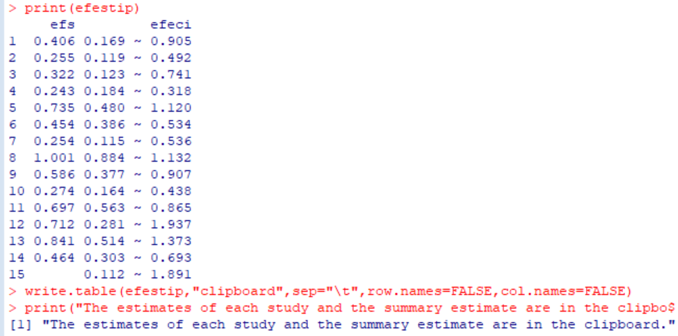
print(efestip)
write.table(efestip,"clipboard",sep="\t",row.names=FALSE,col.names=FALSE)
print("The estimates of each study and the summary estimate are in the clipboard.")
##########
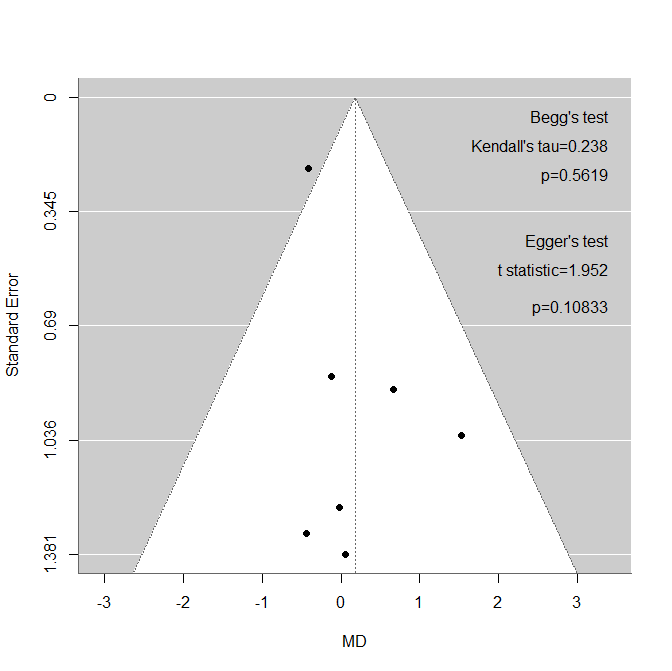
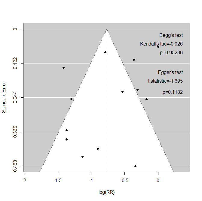
metaforのfunnel()関数、regtest()、ranktest()関数を用いて、Funnel plot作成と、Beggの検定、Eggerの検定を実行するスクリプトを作成しました。Forest plotが出力された後で、実行してください。
Funnel plot作成用のスクリプト
########################
library(metafor)

#Plot funnel plot.
if(em == "MD"){
yi = md
vi=1/weights
sei = sqrt(1/weights)
mu = mu_md
dev.new(width=7,height=7)
funnel(yi, sei = sei, level = c(95), refline = mu,xlab = "MD", ylab = "Standard Error")
}
if(em == "SMD"){
yi = smd
vi=1/weights
sei = sqrt(1/weights)
mu = mu_smd
dev.new(width=7,height=7)
funnel(yi, sei = sei, level = c(95), refline = mu,xlab = "SMD", ylab = "Standard Error")
}

#Asymmetry test with Egger and Begg's tests.
egger=regtest(yi, sei=sei,model="lm", ret.fit=FALSE)
begg=ranktest(yi, vi)

#Print the results to the console.
print("Egger's test:")
print(egger)
print("Begg's test")
print(begg)

#Add Begg and Egger to the plot.
fsfn=1
em=toString(exdat$label[6])
outyes=toString(exdat$label[4])
funmax=par("usr")[3]-par("usr")[4]
gyou=funmax/12
fxmax=par("usr")[2]-(par("usr")[2]-par("usr")[1])/40
text(fxmax,gyou*0.5,"Begg's test",pos=2,cex=fsfn)
kentau=toString(round(begg$tau,digits=3))
text(fxmax,gyou*1.2,paste("Kendall's tau=",kentau,sep=""),pos=2,cex=fsfn)
kenp=toString(round(begg$pval,digits=5))
text(fxmax,gyou*1.9,paste("p=",kenp,sep=""),pos=2,cex=fsfn)

text(fxmax,gyou*3.5,"Egger's test",pos=2,cex=fsfn)
tstat=toString(round(egger$zval,digits=3))
text(fxmax,gyou*4.2,paste("t statistic=",tstat,sep=""),pos=2,cex=fsfn)
tstap=toString(round(egger$pval,digits=5))
text(fxmax,gyou*5.1,paste("p=",tstap,sep=""),pos=2,cex=fsfn)
#####################################