前の投稿で、Google NotebookLMで、PubMed検索結果をAbstract (text)形式でテキストファイルとしてダウンロードしそれを400件ずつのテキストファイルに分割しソースとしてアップロードして、PICO要約表の作成ができることを、解説しました。その際は、ソースファイルを1つずつ選択して、文献選定とPICO要約表の作成のためのプロンプトを実行した後、更新をしてから、次のソースファイルで同じことを繰り返し処理させることで、1894件の文献ソースから採用基準・除外基準に合致するランダム化比較試験が11件に絞られ、標的文献9件をすべて選定できました。

NotebookLMでは分析対象のソースファイルにチェックを入れることで、1つのソースファイルを選んでプロンプトを実行することができるので、操作を連続してスムーズに進めることができるのがGeminiに対する利点と言えます。
今回、Geminiではどうか試してみることにしました。Google Workspace Business Standardを契約しているので、100万トークン(英語ワードで約75万語)まで処理できます。(無料版では3.2万トークンまでなので、残念ながら同じことをするのは無理です。)Gemini 3ではなく、Gemini PRO 2.5 高速モードを使いました。
Geminiの場合も左上のチャットを新規作成をクリックして毎回更新してから、それぞれのAbstract (text)形式のテキストファイルをアップロードして、それに続けて以下のプロンプトを実行します。
ソースのテキストファイルから、以下の採用基準と除外基準に合致する文献を抽出して、Study ID、P、I、C、O、コメント、PMIDの7列からなるテーブルを作成してください。P,I,C,O,コメントは原則日本語で記述してください。研究は年度の新しい順に並べ、Googleスプレッドシートへエクスポートできるテーブルとして提示してください。
Study IDは第一著者の姓のフルスペル+半角スペース+イニシャル+半角スペース+年度を記述してください。著者名が複数の場合et al.を付ける必要はありません。
Pの欄は対象者に関する記述(症例数)、Iの欄は介入に関する記述(症例数)、Cの欄は対照の治療に関する記述(症例数)、Oの欄は測定されたアウトカムの内容を記述してください。
コメント蘭は介入の効果の概略を記述してください。
PMIDの欄はhttps://pubmed.ncbi.nlm.nih.gov/PMID/のように、クリックしたらPubMedの該当する文献を開けるようなリンクのURLを記述してください。URLの最後は/で閉じてください。"PMID"は不要で、URLだけを記述してください。
P, I, C, Oの欄は他の研究との違いが分かる程度の詳細な情報を含めてください。
単位の表記はLaTex記法を使わないでテキストで表示してください。

採用基準:
研究デザインはランダム化比較試験。
対象は肝細胞癌患者。
介入がタモキシフェン単独投与。
対照がプラセボあるいは無治療あるいは保存的治療。
生存をアウトカムとして分析。
除外基準:
システマティックレビュー/メタアナリシスの論文。
対照が肝動脈塞栓療法や化学塞栓療法の研究。
対照でタモキシフェンが投与されている研究。
アウトカムとして生存が分析されていない研究。
まず、左サイドバーのチャットを新規作成の部分をクリックして、チャットを新規作成します。

ソースファイルをチャットエリアにドラグアンドドロップして読み込ませてから、プロンプトを書き込んで、実行します(Enterキーまたは>ボタンをクリック)。
回答では、ファイル1からは該当する文献はありませんでしたが、システマティックレビュー/メタアナリシスの論文(今回基準としたNaing C 2024)があることを述べています。

ここで、プロンプトを実行後、左のサイドバーにプロンプトの履歴が現れますので、左サイドバーの一番上のチャット名を選択して、削除します。なお、左サイドバーのチャットの一覧では、右側に内容が表示されているチャットはハイライトされていますので、削除したいファイルの内容を確認できます。

チャットを削除しますかの確認画面で削除をクリックします。

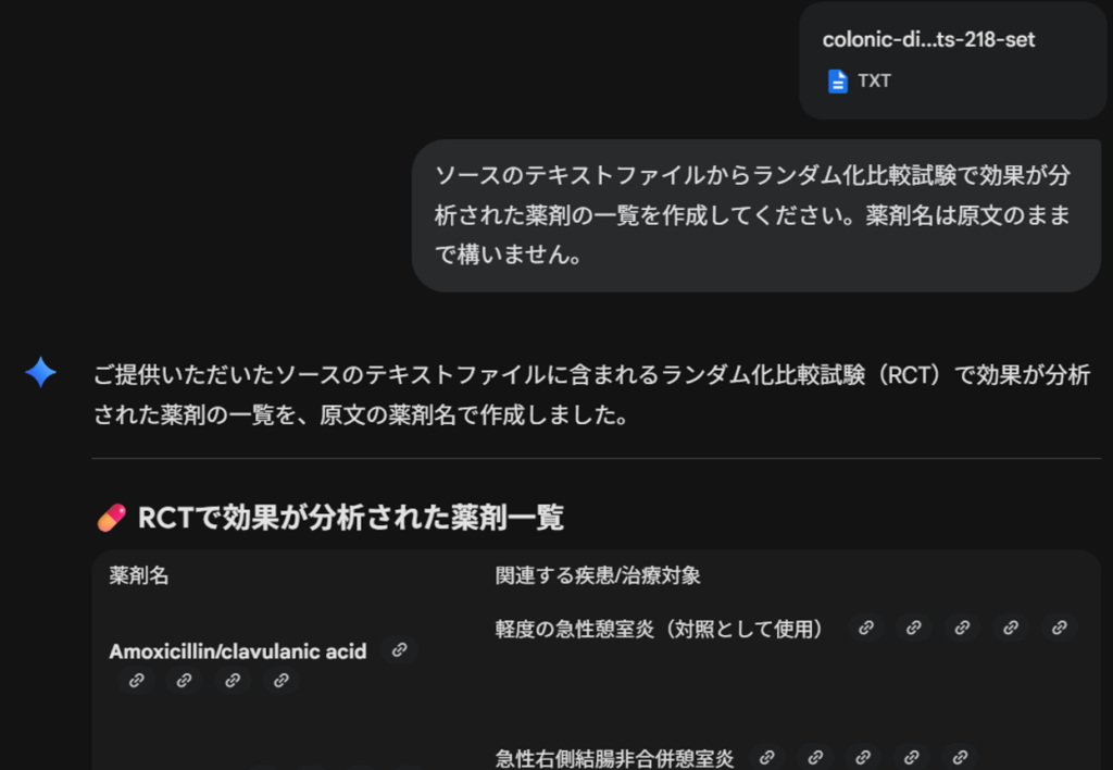
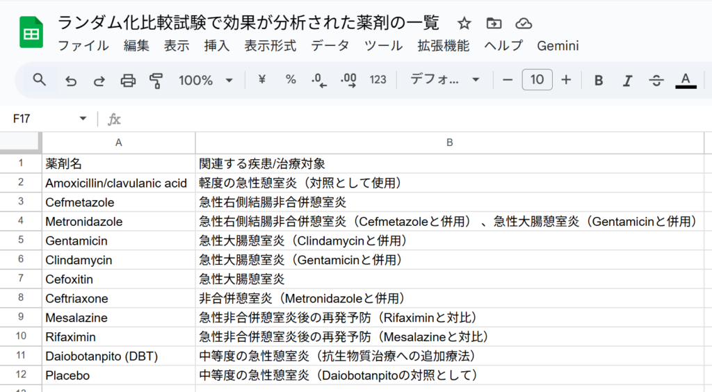
再度、チャットを新規作成し、ファイル2をアップロードして、同じプロンプトを実行します。”該当する文献は見つかりませんでした”と回答が提示され、各文献で使用されていた薬剤名の一覧が表示されました。
ファイル2のチャットの履歴も削除して、チャットを新規作成し、ファイル3をアップロードして、同じプロンプトを実行します。”該当する文献は見つかりませんでした”と回答が提示され、評価された薬剤名に関する言及と、参考情報として、”なお、ソーステキストには、タモキシフェンに関する以下の言及が含まれており、HCC治療における役割が否定されています。タモキシフェンはHCCの治療において役割がないと結論づけられた 。HCCの治療としてタモキシフェンは役割がないという言及がある 。”と記述されていました。このような情報も有用かと思います。
ファイル3のチャットの履歴も削除して、チャットを新規作成し、ファイル4をアップロードして、同じプロンプトを実行します。2件の文献が選定され、いずれも標的文献に含まれていた文献でした。

PMIDのリンクが有効なので、クリックするとPubMedの該当論文のアブストラクトがブラウザで表示されます。ここで、採用基準に合致していることを確認することもできます。まずはすべての文献をスプレッドシートに貼り付けようと思います。表の部分ではなく、左下のコピー用のボタンをクリックして、Googleスプレッドシートに貼り付けます。Excelにも貼り付けられます。どちらも、体裁を整える必要がありますが、まずは不要な行を削除して、左上上角をクリックして、シート全体を選択してから、フォントサイズを11か10に変更し、表示形式のメニューから配置を左、上、そしてラッピングから折り返すを選択し、列幅も調整します。一か所LaTex記法の表示が残っていたのでマニュアルで変更しました。
ファイル4のチャットの履歴も削除して、チャットを新規作成し、ファイル5をアップロードして、同じプロンプトを実行します。9件の文献が選定されましたが、年度の新しい順になっていなかったので、そのまま続けて、プロンプト”表を年度の新しい順に並べ替えてください。”を実行してみましたが、一文献だけ順序がずれていたので、全部をGoogleスプレッドシートに貼り付けてから、並べ替えることにしました。
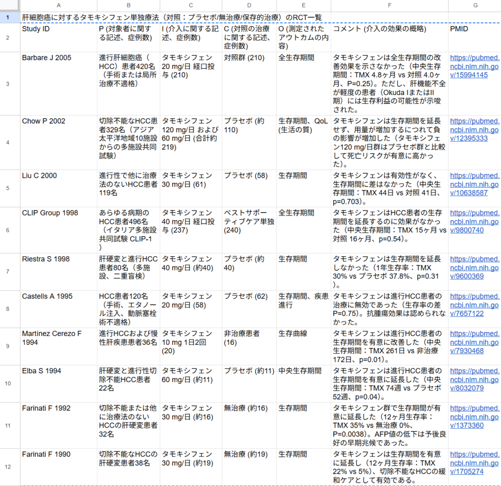
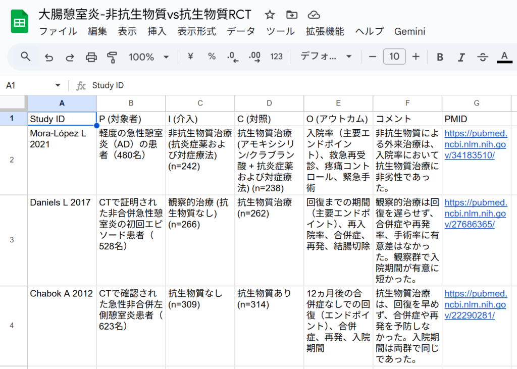
ファイル4と5から計11件の文献が選定され、基準としてNaing C 2024のコクランシステマティックレビューで採用論文として選定されていた9件はすべて含まれていました。スプレッドシートで作成したPICO要約表を図として以下に示します。Study IDのシアンで色を付けてある文献が標的文献です。

400文献ずつに分割してプロンプト実行ごとに履歴を削除して新規チャットとして繰り返し実行した場合は、漏れなく必要な文献が選定されました。追加されたPerrone F 2002はCLIP Group 1998で報告された試験と同じ内容で後で報告されたものでした。Farinati Fの1990と1992の2件は同じ研究なのかどうかをチェックする必要があります。
今回の検討からは、Gemini PRO 2.5 高速モードでも、小さいファイルに分割して、一つ一つ新規チャットにして選定作業を行えば、十分実用的なレベルで文献の一次選定とPICO要約表を作成できそうなことが分かりました。
なお、ファイル4と5の単語数は合計約19万です。この2つのファイルをアップロードして同じプロンプトを実行したところ、結果は11件で基準に合致しない文献が4件含まれていました。さらにファイル3,4,5を合わせると32万語になり、アップロードできないというメッセージがでました。やはり、一度に処理するテキストの容量に限度があるようです。
また、Copilot (GPT-5)で、ファイル4をアップロードして同じプロンプトを実行したところ、5件が選定され、1件は非適格文献で、400件程度の文献数ではうまく処理できないようでした。
今回は400件ずつに分割してファイルひとつずつ選定作業を行えば、Geminiでも文献の一次選定とPICO要約表の作成が出来そうなことが分かりました。
大きなサイズのAbstract (text)形式のテキストファイルを分割する方法については、前回の投稿を参照してください。